Live Case: S&P500 (2 of 3)

Aug 7, 2023

# Load the required libraries, suppressing annoying startup messages
library(dplyr, quietly = TRUE, warn.conflicts = FALSE)
library(tibble, quietly = TRUE, warn.conflicts = FALSE)
library(ggplot2, quietly = TRUE, warn.conflicts = FALSE) # For data visualization
library(ggpubr, quietly = TRUE, warn.conflicts = FALSE) # For data visualization

library(gsheet, quietly = TRUE, warn.conflicts = FALSE) 
library(rmarkdown, quietly = TRUE, warn.conflicts = FALSE) 
library(knitr, quietly = TRUE, warn.conflicts = FALSE) 
library(kableExtra, quietly = TRUE, warn.conflicts = FALSE)

ISSUE: Understanding the S&P500 as a whole Aug 06, 2023 -=- This chapter is being heavily edited

S&P 500 Data - PRELIMINARY SETUP

We will continue our analysis of the S&P 500. Load the data, as described in the chapter Live Case: S&P500 (1 of 3)

# Read S&P500 stock data present in a Google Sheet.
library(gsheet)
prefix <- "https://docs.google.com/spreadsheets/d/"
sheetID <- "11ahk9uWxBkDqrhNm7qYmiTwrlSC53N1zvXYfv7ttOCM"
url500 <- paste(prefix,sheetID) # Form the URL to connect to
sp500 <- gsheet2tbl(url500) # Read it into a tibble called sp500

Rename columns, as described in the chapter Live Case: S&P500 (1 of 3).

suppressPackageStartupMessages(library(dplyr))

# Define a mapping of new column names
new_names <- c(
  "Date", "Stock", "StockName", "Sector", "Industry", 
  "MarketCap", "Price", "Low52Wk", "High52Wk", 
  "ROE", "ROA", "ROIC", "GrossMargin", 
  "OperatingMargin", "NetMargin", "PE", 
  "PB", "EVEBITDA", "EBITDA", "EPS", 
  "EBITDA_YOY", "EBITDA_QYOY", "EPS_YOY", 
  "EPS_QYOY", "PFCF", "FCF", 
  "FCF_QYOY", "DebtToEquity", "CurrentRatio", 
  "QuickRatio", "DividendYield", 
  "DividendsPerShare_YOY", "PS", 
  "Revenue_YOY", "Revenue_QYOY", "Rating"
)
# Rename the columns using the new_names vector
sp500 <- sp500 %>% 
  rename_with(~ new_names, everything())

Remove Rows containing no data or Null values, as described in the chapter Live Case: S&P500 (1 of 3).

# Check for blank or null values in the "Stock" column
hasNull <- any(sp500$Stock == "" | is.null(sp500$Stock))
if (hasNull) { 
    # Remove rows with null or blank values from the dataframe tibble
    sp500 <- sp500[!(is.null(sp500$Stock) | sp500$Stock == ""), ]
}

The S&P500 shares are divided into multiple Sectors. Thus, model Sector as a factor() variable, as described in the chapter Live Case: S&P500 (1 of 3).

sp500$Sector <- as.factor(sp500$Sector)

Stock Ratings: The S&P500 shares have Technical Ratings such as {Buy, Sell, ..}. Model the data column Rating as a factor() variable, as described in the chapter Live Case: S&P500 (1 of 3).

sp500$Rating <- as.factor(sp500$Rating)

Low52WkPerc: Create a new column to track Share Prices relative to their 52 Week Low, as described in the chapter Live Case: S&P500 (1 of 3).

sp500 <- sp500 %>% mutate(Low52WkPerc = round((Price - Low52Wk)*100 / Low52Wk,2))
colnames(sp500)

 [1] "Date"                  "Stock"                 "StockName"            
 [4] "Sector"                "Industry"              "MarketCap"            
 [7] "Price"                 "Low52Wk"               "High52Wk"             
[10] "ROE"                   "ROA"                   "ROIC"                 
[13] "GrossMargin"           "OperatingMargin"       "NetMargin"            
[16] "PE"                    "PB"                    "EVEBITDA"             
[19] "EBITDA"                "EPS"                   "EBITDA_YOY"           
[22] "EBITDA_QYOY"           "EPS_YOY"               "EPS_QYOY"             
[25] "PFCF"                  "FCF"                   "FCF_QYOY"             
[28] "DebtToEquity"          "CurrentRatio"          "QuickRatio"           
[31] "DividendYield"         "DividendsPerShare_YOY" "PS"                   
[34] "Revenue_YOY"           "Revenue_QYOY"          "Rating"               
[37] "Low52WkPerc"

Well done! Our data is now ready for analysis!!

Low52WkPerc: Create a new column MarketCapBillions = MarketCap/1000,000,000, as described in the chapter Live Case: S&P500 (1 of 3).

sp500 <- sp500 %>% mutate(MarketCapBillions = round(MarketCap/1000000000))
colnames(sp500)

 [1] "Date"                  "Stock"                 "StockName"            
 [4] "Sector"                "Industry"              "MarketCap"            
 [7] "Price"                 "Low52Wk"               "High52Wk"             
[10] "ROE"                   "ROA"                   "ROIC"                 
[13] "GrossMargin"           "OperatingMargin"       "NetMargin"            
[16] "PE"                    "PB"                    "EVEBITDA"             
[19] "EBITDA"                "EPS"                   "EBITDA_YOY"           
[22] "EBITDA_QYOY"           "EPS_YOY"               "EPS_QYOY"             
[25] "PFCF"                  "FCF"                   "FCF_QYOY"             
[28] "DebtToEquity"          "CurrentRatio"          "QuickRatio"           
[31] "DividendYield"         "DividendsPerShare_YOY" "PS"                   
[34] "Revenue_YOY"           "Revenue_QYOY"          "Rating"               
[37] "Low52WkPerc"           "MarketCapBillions"

ANALYSIS OF S&P500 SECTORS

The table() function allows us to count how many stocks are part of each sector.

tab<- addmargins(table(sp500$Sector))
kable(tab)

Var1	Freq
Commercial Services	13
Communications	3
Consumer Durables	12
Consumer Non-Durables	32
Consumer Services	29
Distribution Services	9
Electronic Technology	49
Energy Minerals	16
Finance	92
Health Services	12
Health Technology	47
Industrial Services	9
Non-Energy Minerals	7
Process Industries	24
Producer Manufacturing	31
Retail Trade	22
Technology Services	50
Transportation	15
Utilities	31
Sum	503

The S&P500 consists of 503 stocks, divided across 19 sectors.

ggplot(data = sp500, 
       aes(y = Sector)) + 
  geom_bar(aes(fill = Sector)) +
  geom_text(stat='count', 
            aes(label=after_stat(count))) +
  labs(title = "Stocks by Sector", 
       x = "No. of Stocks", 
       y = "Sector")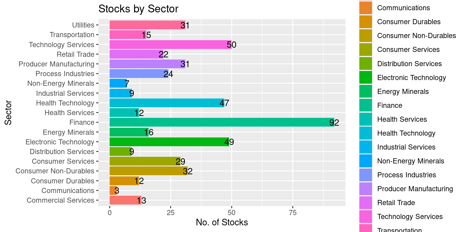

Numbers of shares by Rating

tab<- addmargins(table(sp500$Rating))
kable(tab)

Var1	Freq
Buy	133
Neutral	36
Sell	146
Strong Buy	158
Strong Sell	30
Sum	503

Pie Chart Showing Proportion of shares by Rating

library(ggpubr)

# Compute counts and proportions of each cylinder type
Rating_counts <- as.data.frame(table(sp500$Rating))
colnames(Rating_counts) <- c("Rating", "n")

# Calculate proportions
Rating_counts$prop <- Rating_counts$n / sum(Rating_counts$n)

# Create labels that display proportions as percentages
Rating_counts$labels <- paste0(round(Rating_counts$prop*100, 2), "%")

# Create the pie chart with proportions
ggpie(data = Rating_counts, 
      x = "prop", 
      fill = "Rating", 
      label = "labels", 
      palette = "jco", 
      title = "Pie Chart of Rating")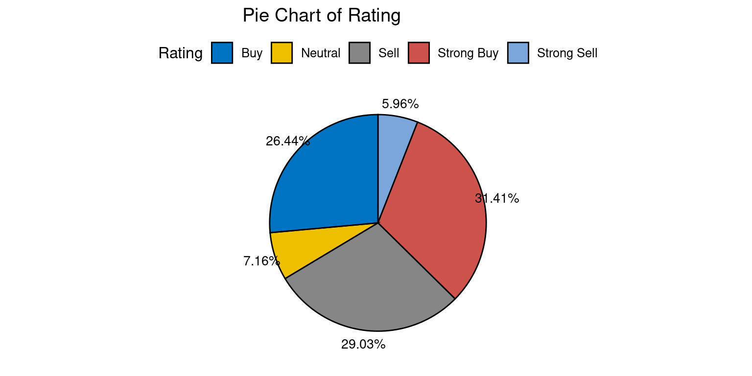

Count Shares by Sector*Rating

tab<- addmargins(table(Sector = sp500$Sector, Rating = sp500$Rating))
kable(tab)

	Buy	Neutral	Sell	Strong Buy	Strong Sell	Sum
Commercial Services	4	1	5	3	0	13
Communications	1	1	0	0	1	3
Consumer Durables	4	0	3	4	1	12
Consumer Non-Durables	4	2	15	10	1	32
Consumer Services	7	5	7	8	2	29
Distribution Services	3	0	2	4	0	9
Electronic Technology	13	1	16	17	2	49
Energy Minerals	7	1	1	5	2	16
Finance	27	6	24	34	1	92
Health Services	4	0	4	3	1	12
Health Technology	9	3	24	6	5	47
Industrial Services	1	0	1	7	0	9
Non-Energy Minerals	3	1	1	2	0	7
Process Industries	6	4	9	4	1	24
Producer Manufacturing	8	0	4	18	1	31
Retail Trade	8	3	5	6	0	22
Technology Services	11	4	20	7	8	50
Transportation	6	2	2	2	3	15
Utilities	7	2	3	18	1	31
Sum	133	36	146	158	30	503

MARKET CAP

TODO: Work in Billions; 1. Market Cap of all companies by Sector

library(janitor)  # This package helps us auto generate the total at the bottom of a table. 
library(kableExtra)

# Market Cap by Sector
MCap <- sp500 %>%
  group_by(Sector) %>%
  summarise(
    MarketCapCr = sum(na.omit(MarketCap)/10000000))

# Total Market Cap of the entire S&P 500 (in Millions)
SP500MarketCap <- sum(sp500$MarketCap/10000000)

# calculating % market cap
PercentMarketCap <- round(MCap$MarketCapCr*100/SP500MarketCap,2)
MCapTab <- cbind(MCap,PercentMarketCap)

# sorting by PercentMarketCap
MCapTab <- MCapTab %>% arrange(desc(PercentMarketCap))

# Use package janitor to add sums at the bottom of the table
MCapTab <- MCapTab %>%   
  adorn_totals("row")

# Use package knittr to format the appearance of the table
MCapTab <- knitr::kable(MCapTab, "html") %>% kable_styling() 
MCapTab

Sector	MarketCapCr	PercentMarketCap
Technology Services	977771.00	23.38
Electronic Technology	657795.29	15.73
Finance	487711.71	11.66
Health Technology	392561.17	9.38
Retail Trade	324468.26	7.76
Consumer Non-Durables	207586.48	4.96
Energy Minerals	148491.47	3.55
Consumer Services	139457.83	3.33
Producer Manufacturing	136313.77	3.26
Commercial Services	130902.32	3.13
Consumer Durables	114063.38	2.73
Utilities	97714.24	2.34
Health Services	91056.18	2.18
Process Industries	78141.93	1.87
Transportation	64189.17	1.53
Communications	41914.50	1.00
Industrial Services	41597.39	0.99
Distribution Services	30238.98	0.72
Non-Energy Minerals	20935.45	0.50
Total	4182910.54	100.00

TODO: Work in Billions; Show “Sum”, “Median”, “Mean” Delete Q1, Q3 all others 2. Summary Statistics of Market Cap (in Cr of USD) by each Sector of S&P500

SectorMC <- sp500 %>%
  group_by(Sector) %>%
  summarise(
    Mean = mean(na.omit(MarketCap/10000000)),
    Median= sd(na.omit(MarketCap/10000000)),
    Median= median(na.omit(MarketCap/10000000)),
    Q1 = quantile(na.omit(MarketCap/10000000), probs = 0.25, na.rm = TRUE),
    Q3 = quantile(na.omit(MarketCap/10000000), probs = 0.75, na.rm = TRUE),
    Min = min(na.omit(MarketCap/10000000)),
    max = max(na.omit(MarketCap/10000000))
  )

tab <- cbind(Sector = SectorMC$Sector, round(SectorMC[,2:7],2))

SMcap <- knitr::kable(tab, "html") %>% kable_styling() 
SMcap

Sector	Mean	Median	Q1	Q3	Min	max
Commercial Services	10069.41	3267.60	1548.76	7075.75	799.37	49231.40
Communications	13971.50	14310.60	12538.50	15574.05	10766.40	16837.50
Consumer Durables	9505.28	1874.35	1345.57	4080.71	748.59	87614.90
Consumer Non-Durables	6487.08	4002.33	1828.88	5986.15	704.24	36477.60
Consumer Services	4808.89	1956.52	1459.00	5360.23	735.13	20752.30
Distribution Services	3359.89	3132.05	2109.38	3554.92	972.20	7748.67
Electronic Technology	13424.39	4055.77	1890.92	7863.17	848.90	274756.00
Energy Minerals	9280.72	5314.84	2656.84	6644.05	1320.63	47445.80
Finance	5301.21	2499.88	1585.23	5005.07	436.14	80651.20
Health Services	7588.02	3780.36	1710.52	7473.15	792.41	44796.10
Health Technology	8352.37	3361.24	1728.29	10788.55	505.77	56161.20
Industrial Services	4621.93	3856.95	3703.41	4758.81	2944.49	8754.51
Non-Energy Minerals	2990.78	2856.22	2195.89	3629.07	597.27	5832.03
Process Industries	3255.91	1696.74	1339.25	3750.41	511.36	19020.10
Producer Manufacturing	4397.22	3357.60	1291.95	5361.67	402.60	14414.60
Retail Trade	14748.56	3637.82	2122.68	10276.64	705.74	148488.00
Technology Services	19555.42	3462.30	1676.70	11599.22	424.51	251646.00
Transportation	4279.28	2530.56	1606.72	5458.89	500.76	13746.80
Utilities	3152.07	2249.51	1778.34	3607.82	891.77	14209.70

Top 10 companies having highest Market Cap

Top10 <- sp500 %>% arrange(desc(MarketCap)) %>% head(10)
Top10 <- Top10[,c(1:4, 6,10:13)]

Top10 <- knitr::kable(Top10, "html") %>% kable_styling() 
Top10

Date	Stock	StockName	Sector	MarketCap	ROE	ROA	ROIC	GrossMargin
9/22/2023	AAPL	Apple Inc.	Electronic Technology	2.74756e+12	160.1	28.2	60.9	43.4
9/22/2023	MSFT	Microsoft Corporation	Technology Services	2.51646e+12	38.8	18.6	28.1	68.9
9/22/2023	GOOG	Alphabet Inc.	Technology Services	1.74660e+12	23.3	16.5	21.2	55.4
9/22/2023	GOOGL	Alphabet Inc.	Technology Services	1.74660e+12	23.3	16.5	21.2	55.4
9/22/2023	AMZN	Amazon.com, Inc.	Retail Trade	1.48488e+12	8.7	2.9	4.6	45.5
9/22/2023	NVDA	NVIDIA Corporation	Electronic Technology	1.12585e+12	40.2	22.2	29.0	64.6
9/22/2023	TSLA	Tesla, Inc.	Consumer Durables	8.76149e+11	28.0	15.4	25.5	21.5
9/22/2023	BRK.B	Berkshire Hathaway Inc. New	Finance	8.06512e+11	17.4	8.9	13.9	19.2
9/22/2023	META	Meta Platforms, Inc.	Technology Services	8.02237e+11	17.4	12.0	14.5	79.4
9/22/2023	LLY	Eli Lilly and Company	Health Technology	5.61612e+11	66.3	12.8	24.8	77.8

PRICE RELATIVE TO 52 WEEK LOW

Summary Statistics of Low52WkPerc by Sector

SM <- sp500 %>%
  group_by(Sector) %>%
  summarise(
    Mean = mean(na.omit(Low52WkPerc)),
    Median= sd(na.omit(Low52WkPerc)),
    Median= median(na.omit(Low52WkPerc)),
    Q1 = quantile(na.omit(Low52WkPerc), probs = 0.25, na.rm = TRUE),
    Q3 = quantile(na.omit(Low52WkPerc), probs = 0.75, na.rm = TRUE),
    Min = min(na.omit(Low52WkPerc)),
    Max = max(na.omit(Low52WkPerc))
  )

tab <- cbind(Sector = SM$Sector, round(SM[,2:7],2))

tab <- tab %>% arrange(Median)

SM <- knitr::kable(tab, "html") %>% kable_styling() 
SM

Sector	Mean	Median	Q1	Q3	Min	Max
Utilities	16.42	10.50	6.69	18.53	2.96	58.01
Consumer Non-Durables	14.79	10.88	5.75	21.57	0.87	40.02
Communications	11.96	12.69	10.66	13.63	8.63	14.57
Health Technology	24.51	17.41	8.19	30.27	0.34	99.76
Transportation	25.10	17.42	5.72	40.53	2.11	81.11
Health Services	24.17	18.05	10.53	33.33	5.81	54.55
Finance	25.46	22.15	13.07	33.97	0.55	102.73
Retail Trade	24.93	22.20	9.98	30.38	0.60	77.76
Process Industries	26.63	25.62	14.23	37.96	3.56	51.92
Distribution Services	27.54	27.29	25.40	34.92	3.37	44.12
Producer Manufacturing	44.69	32.95	23.12	61.69	1.76	139.34
Electronic Technology	44.70	35.11	15.35	53.44	2.58	321.74
Industrial Services	45.48	35.64	24.79	79.90	8.13	82.25
Commercial Services	37.54	36.78	23.90	49.26	12.57	71.65
Energy Minerals	40.83	38.41	31.45	49.98	15.68	74.72
Consumer Services	46.97	39.47	26.29	50.99	5.89	170.46
Technology Services	48.15	40.03	23.82	62.88	6.98	253.80
Consumer Durables	53.57	40.06	14.22	69.92	8.36	171.12
Non-Energy Minerals	38.67	46.13	26.74	52.44	5.33	60.84

Sector Communications and Utilities are closest to its 52 week low.

Box Plot for Low52WkPerc by Sector TODO: Truncate at 100; Rotate by 90 degrees; Sort Sectors by Median(Low52WkPerc)

library(ggplot2)

ggplot(sp500, aes(Sector, Low52WkPerc)) + geom_boxplot() +
  theme(axis.text.x = element_text(angle = 45, vjust = 1, hjust = 1))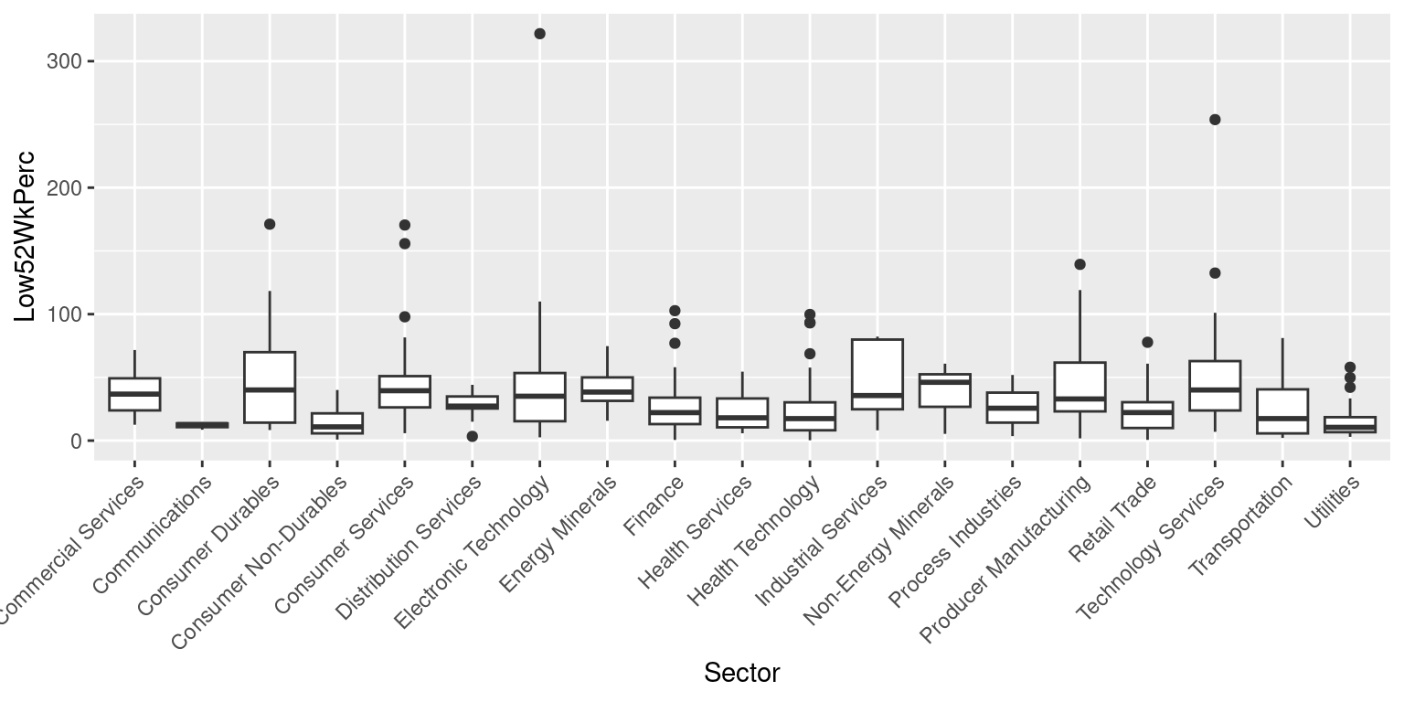

PROFITABILITY BY SECTOR

ROE

Summary Statistics of ROE by each Sector of S&P500

SectorROE <- sp500 %>%
  group_by(Sector) %>%
  summarise(
    Mean = mean(na.omit(ROE)),
    Median= sd(na.omit(ROE)),
    Median= median(na.omit(ROE)),
    Q1 = quantile(na.omit(ROE), probs = 0.25, na.rm = TRUE),
    Q3 = quantile(na.omit(ROE), probs = 0.75, na.rm = TRUE),
    Min = min(na.omit(ROE)),
    max = max(na.omit(ROE))
  )

cbind(Sector = SectorROE$Sector, round(SectorROE[,2:7],2))

                   Sector   Mean Median    Q1    Q3     Min    max
1     Commercial Services  37.98  26.40 16.40 43.60     3.5  175.2
2          Communications   8.10   9.10  0.55 16.15    -8.0   23.2
3       Consumer Durables  12.42  17.75  6.85 25.38   -51.4   45.2
4   Consumer Non-Durables 129.60  19.60  6.40 34.60   -11.5 2878.8
5       Consumer Services  31.11   9.40  1.43 42.88  -185.6  359.9
6   Distribution Services  81.10  34.20 22.15 56.45     5.1  371.2
7   Electronic Technology  31.65  18.75  8.10 36.80   -14.8  160.1
8         Energy Minerals  43.12  26.95 23.78 41.45    18.0  230.2
9                 Finance  21.52  10.95  7.62 16.67   -39.2  714.3
10        Health Services  20.63  17.30 12.05 24.05     8.3   56.0
11      Health Technology  19.87  13.10  6.80 22.73   -49.3  173.5
12    Industrial Services  21.04  22.60 10.70 31.10     7.7   36.5
13    Non-Energy Minerals  13.84  13.50  3.40 21.80    -3.8   36.8
14     Process Industries  25.72  18.60 15.35 24.62   -13.2  125.5
15 Producer Manufacturing  24.26  19.40 12.80 29.40   -13.6   95.9
16           Retail Trade  74.36  28.75 14.47 44.00 -1224.5 2065.3
17    Technology Services  33.28  18.00 10.70 32.65   -70.6  416.6
18         Transportation  36.34  33.50 20.85 49.08     4.1  104.4
19              Utilities   8.12   8.70  7.65 10.60   -47.6   35.5

Box Plot for ROE by Sector

library(ggplot2)

ggplot(sp500, aes(Sector, ROE)) + geom_boxplot() +
  theme(axis.text.x = element_text(angle = 45, vjust = 1, hjust = 1))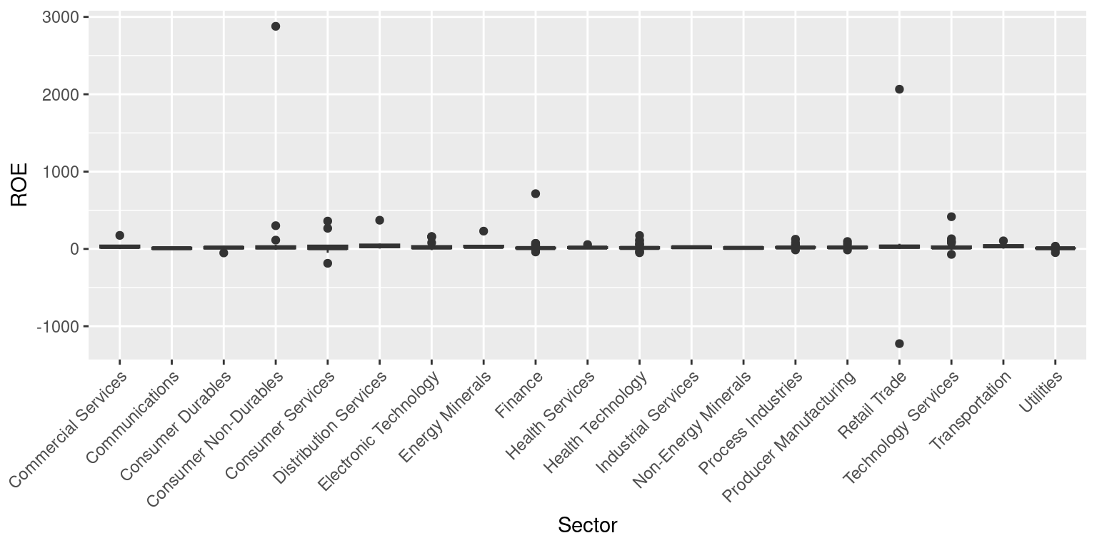

ROA

Summary Statistics of ROA by each Sector of S&P500

SectorROA <- sp500 %>%
  group_by(Sector) %>%
  summarise(
    Mean = mean(na.omit(ROA)),
    Median= sd(na.omit(ROA)),
    Median= median(na.omit(ROA)),
    Q1 = quantile(na.omit(ROA), probs = 0.25, na.rm = TRUE),
    Q3 = quantile(na.omit(ROA), probs = 0.75, na.rm = TRUE),
    Min = min(na.omit(ROA)),
    max = max(na.omit(ROA))
  )

cbind(Sector = SectorROA$Sector, round(SectorROA[,2:7],2))

                   Sector  Mean Median    Q1    Q3   Min  max
1     Commercial Services 10.25   6.20  5.30 18.10   1.7 27.2
2          Communications  2.13   2.90  0.40  4.25  -2.1  5.6
3       Consumer Durables  8.75   9.70  1.13 15.53  -8.8 27.9
4   Consumer Non-Durables  7.15   6.60  3.10 10.75  -5.9 18.9
5       Consumer Services  6.38   3.20  0.80 13.30  -6.6 29.0
6   Distribution Services  9.79   5.90  2.90 15.50   0.6 24.5
7   Electronic Technology  9.46   8.80  3.90 13.60  -6.7 28.2
8         Energy Minerals 14.32  14.15 11.70 15.98   7.4 21.9
9                 Finance  3.28   2.40  1.10  4.23  -2.9 24.1
10        Health Services  5.74   5.50  4.27  6.62   2.7 11.0
11      Health Technology  6.66   6.70  2.95 10.70 -30.8 28.9
12    Industrial Services  6.58   5.70  4.20  9.00   3.3 10.6
13    Non-Energy Minerals  7.10   5.20  1.05 11.70  -2.2 21.2
14     Process Industries  7.01   6.25  5.32  7.43  -5.0 24.8
15 Producer Manufacturing  9.02   8.70  5.15 10.90  -3.1 25.1
16           Retail Trade  8.84   8.80  5.38 13.65 -23.2 24.8
17    Technology Services  9.27   8.65  5.15 13.75 -35.4 41.5
18         Transportation  8.75   7.90  3.95 10.70   1.1 26.2
19              Utilities  2.33   2.30  2.00  3.20  -6.5  5.6

Box Plot for ROA by Sector

library(ggplot2)

ggplot(sp500, aes(Sector, ROA)) + geom_boxplot() +
  theme(axis.text.x = element_text(angle = 45, vjust = 1, hjust = 1))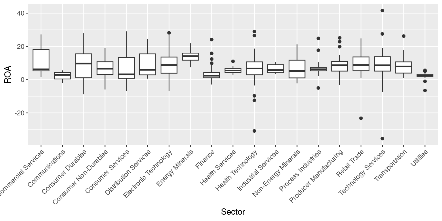

Live Case: S&P500 (2b of 3)

Aug 06, 2023 -=- This chapter is being heavily edited

ISSUE: Analysis of a particular SECTOR We have chosen to deeply analyze the HEALTH TECHNOLOGY Sector

SECTOR LEVEL ANALYSIS begins here

Filter the data by sector Health Services, and display the number of stocks in the sector

ts <- sp500 %>%
        filter(Sector=='Health Services')

nrow(ts)

[1] 12

There are 12 number of of stocks in the sector Health Services

Select the Specific Coulumns from the filtered dataframe `ts` (Health Services)

ts2 <- ts %>%
        select(Date, Stock, StockName,Sector,  Industry, MarketCap, Price,Low52Wk, High52Wk,
               ROE, ROA,ROIC,GrossMargin, GrossMargin, 
               NetMargin, Rating)

colnames(ts2)

 [1] "Date"        "Stock"       "StockName"   "Sector"      "Industry"   
 [6] "MarketCap"   "Price"       "Low52Wk"     "High52Wk"    "ROE"        
[11] "ROA"         "ROIC"        "GrossMargin" "NetMargin"   "Rating"

Arrange the Dataframe by ROE

ts3 <- ts2 %>% arrange(desc(ROE))

Top 10 Shares in Sector Health Services Based on ROE

head(ts3,10)

# A tibble: 10 × 15
   Date   Stock StockName Sector Industry MarketCap Price Low52Wk High52Wk   ROE
   <chr>  <chr> <chr>     <fct>  <chr>        <dbl> <dbl>   <dbl>    <dbl> <dbl>
 1 9/22/… DVA   DaVita I… Healt… Medical…   8.98e 9  98.3    65.3    117    56  
 2 9/22/… MOH   Molina H… Healt… Managed…   1.91e10 327     256.     374    28.4
 3 9/22/… UNH   UnitedHe… Healt… Managed…   4.48e11 484.    446.     558.   27.2
 4 9/22/… HUM   Humana I… Healt… Managed…   5.84e10 472.    423.     571.   20.9
 5 9/22/… IQV   IQVIA Ho… Healt… Service…   3.90e10 213     166.     242.   19.7
 6 9/22/… ELV   Elevance… Healt… Managed…   1.05e11 444.    412      550.   17.3
 7 9/22/… CI    The Cign… Healt… Managed…   8.39e10 283.    240.     340.   14.6
 8 9/22/… DGX   Quest Di… Healt… Service…   1.43e10 127.    120.     158.   12.5
 9 9/22/… UHS   Universa… Healt… Hospita…   7.92e 9 128.     82.5    159.   11.6
10 9/22/… CNC   Centene … Healt… Managed…   3.66e10  67.6    60.8     87.8  10.4
# ℹ 5 more variables: ROA <dbl>, ROIC <dbl>, GrossMargin <dbl>,
#   NetMargin <dbl>, Rating <fct>

Mutate a data column called (Low52WkPerc), then show top 10 ROE stocks

ts4 <- ts3 %>% mutate(Low52WkPerc = round((Price - Low52Wk)*100 / Low52Wk,2))
head(ts4[,c(1:3,10,16)],10)

# A tibble: 10 × 5
   Date      Stock StockName                         ROE Low52WkPerc
   <chr>     <chr> <chr>                           <dbl>       <dbl>
 1 9/22/2023 DVA   DaVita Inc.                      56         50.5 
 2 9/22/2023 MOH   Molina Healthcare Inc            28.4       27.6 
 3 9/22/2023 UNH   UnitedHealth Group Incorporated  27.2        8.57
 4 9/22/2023 HUM   Humana Inc.                      20.9       11.4 
 5 9/22/2023 IQV   IQVIA Holdings, Inc.             19.7       28.5 
 6 9/22/2023 ELV   Elevance Health, Inc.            17.3        7.86
 7 9/22/2023 CI    The Cigna Group                  14.6       17.8 
 8 9/22/2023 DGX   Quest Diagnostics Incorporated   12.5        5.81
 9 9/22/2023 UHS   Universal Health Services, Inc.  11.6       54.6 
10 9/22/2023 CNC   Centene Corporation              10.4       11.2

Low52WkPerc for all the Health Sector Stocks, as shown below

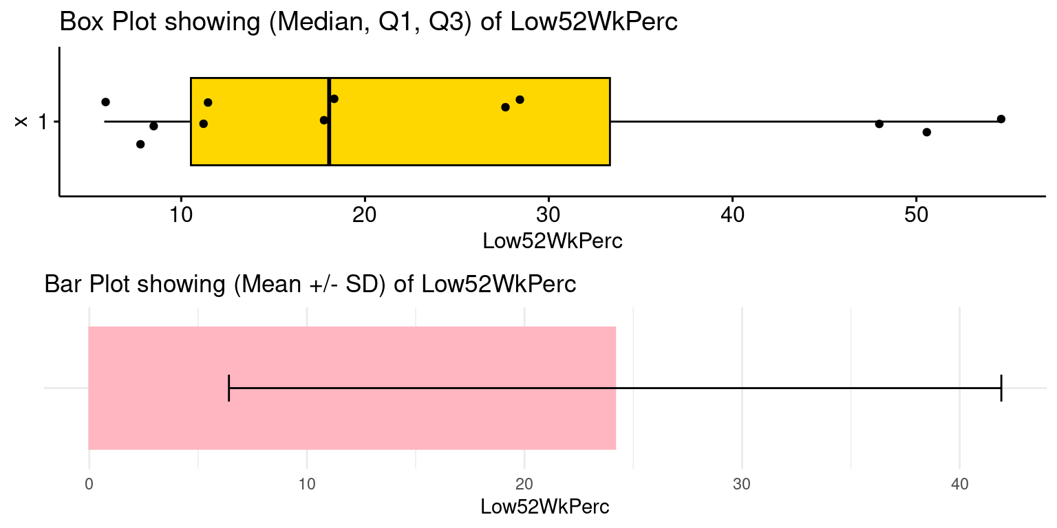
Summary Statistics of ROE

ts3 <- na.omit(ts3)

ROESum <- ts3 %>%
  summarise(
    Mean = mean(ROE),
    Median= sd(ROE),
    Median= median(ROE),
    Q1 = quantile(ROE, probs = 0.25, na.rm = TRUE),
    Q3 = quantile(ROE, probs = 0.75, na.rm = TRUE),
    Min = min(ROE),
    max = max(ROE)
  )

ROESum <- round(ROESum,2)
ROESum

# A tibble: 1 × 6
   Mean Median    Q1    Q3   Min   max
  <dbl>  <dbl> <dbl> <dbl> <dbl> <dbl>
1  21.6   12.5  11.6  19.7   8.3    56

ROE for all the Stocks in Health Sector, as shown below*

Top 10 Shares in Health Sector with highest ROE

ts4 %>% 
  select(Stock, Price, Low52Wk, Low52WkPerc, ROA, ROE) %>% 
  arrange(desc(ROE))%>%
  slice(1:10) %>%
  kable("html", caption = "Top 10 Shares in Health Sector with highest ROE") %>% 
  kable_styling()

Top 10 Shares in Health Sector with highest ROE
Stock	Price	Low52Wk	Low52WkPerc	ROA	ROE
DVA	98.3	65.3	50.54	2.7	56.0
MOH	327.0	256.2	27.63	7.0	28.4
UNH	483.9	445.7	8.57	8.3	27.2
HUM	471.5	423.3	11.39	6.5	20.9
IQV	213.0	165.8	28.47	4.3	19.7
ELV	444.4	412.0	7.86	6.1	17.3
CI	283.3	240.5	17.80	4.5	14.6
DGX	127.4	120.4	5.81	5.9	12.5
UHS	127.5	82.5	54.55	5.1	11.6
CNC	67.6	60.8	11.18	3.3	10.4

ROE versus ROA and colored by Price rel. to 52 Week Low

top10 <- 
  ts4 %>% 
  select(Stock, Price, Low52Wk, Low52WkPerc, ROA, ROE) %>% 
  arrange(desc(ROE))%>%
  slice(1:10)

top10$name <- top10$Stock

ggscatter(top10, 
          x = "ROA", 
          y = "ROE", 
          size = "Low52WkPerc",
          color = "Low52WkPerc",
          alpha = 0.5,
          label = "name", 
          repel = TRUE,
          title = "ROE vs ROA, Low52WkPerc for Health Sector with highest ROE") + 
  gradient_color(c("darkgreen",  "red"))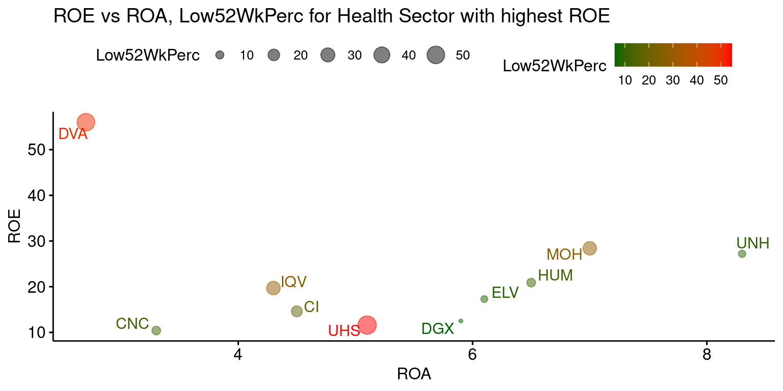

Summary Statistics of All key variables in Sector Health Services

ts3 <- na.omit(ts3)

ROESum <- ts3 %>%
  summarise(
    Mean = mean(ROE),
    Median= sd(ROE),
    Median= median(ROE),
    Q1 = quantile(ROE, probs = 0.25, na.rm = TRUE),
    Q3 = quantile(ROE, probs = 0.75, na.rm = TRUE),
    Min = min(ROE),
    max = max(ROE)
  )

ROESum <- round(ROESum,2)


ROASum <- ts3 %>%
  summarise(
    Mean = mean(ROA),
    Median= sd(ROA),
    Median= median(ROA),
    Q1 = quantile(ROA, probs = 0.25, na.rm = TRUE),
    Q3 = quantile(ROA, probs = 0.75, na.rm = TRUE),
    Min = min(ROA),
    max = max(ROA)
  )

ROASum <- round(ROASum,2)

ROICSum <- ts3 %>%
  summarise(
    Mean = mean(ROIC),
    Median= sd(ROIC),
    Median= median(ROIC),
    Q1 = quantile(ROIC, probs = 0.25, na.rm = TRUE),
    Q3 = quantile(ROIC, probs = 0.75, na.rm = TRUE),
    Min = min(ROIC),
    max = max(ROIC)
  )

ROICSum <- round(ROICSum,2)

GrossMarginSum <- ts3 %>%
  summarise(
    Mean = mean(GrossMargin),
    Median= sd(GrossMargin),
    Median= median(GrossMargin),
    Q1 = quantile(GrossMargin, probs = 0.25, na.rm = TRUE),
    Q3 = quantile(GrossMargin, probs = 0.75, na.rm = TRUE),
    Min = min(GrossMargin),
    max = max(GrossMargin)
  )

GrossMarginSum <- round(GrossMarginSum,2)

NetMarginSum <- ts3 %>%
  summarise(
    Mean = mean(NetMargin),
    Median= sd(NetMargin),
    Median= median(NetMargin),
    Q1 = quantile(NetMargin, probs = 0.25, na.rm = TRUE),
    Q3 = quantile(NetMargin, probs = 0.75, na.rm = TRUE),
    Min = min(NetMargin),
    max = max(NetMargin)
  )

NetMarginSum <- round(NetMarginSum,2)

Metrics <- c("ROE","ROA","ROIC","GrossMargin","NetMargin")

ftab <- rbind(ROESum, ROASum, ROICSum, GrossMarginSum, NetMarginSum)
ftab <- cbind(Metrics, ftab)
ftab

      Metrics  Mean Median   Q1   Q3 Min  max
1         ROE 21.62   12.5 11.6 19.7 8.3 56.0
2         ROA  4.44    4.3  4.2  5.1 2.7  5.9
3        ROIC  5.70    6.0  5.1  6.3 3.7  7.4
4 GrossMargin 23.26   25.5 23.0 27.1 7.9 32.8
5   NetMargin  6.08    5.7  5.0  7.5 3.9  8.3

Summary Statistics of ROE by each Sector of S&P500

SectorROE <- sp500 %>%
  group_by(Sector) %>%
  summarise(
    Mean = mean(na.omit(ROE)),
    Median= sd(na.omit(ROE)),
    Median= median(na.omit(ROE)),
    Q1 = quantile(na.omit(ROE), probs = 0.25, na.rm = TRUE),
    Q3 = quantile(na.omit(ROE), probs = 0.75, na.rm = TRUE),
    Min = min(na.omit(ROE)),
    max = max(na.omit(ROE))
  )

cbind(Sector = SectorROE$Sector, round(SectorROE[,2:7],2))

                   Sector   Mean Median    Q1    Q3     Min    max
1     Commercial Services  37.98  26.40 16.40 43.60     3.5  175.2
2          Communications   8.10   9.10  0.55 16.15    -8.0   23.2
3       Consumer Durables  12.42  17.75  6.85 25.38   -51.4   45.2
4   Consumer Non-Durables 129.60  19.60  6.40 34.60   -11.5 2878.8
5       Consumer Services  31.11   9.40  1.43 42.88  -185.6  359.9
6   Distribution Services  81.10  34.20 22.15 56.45     5.1  371.2
7   Electronic Technology  31.65  18.75  8.10 36.80   -14.8  160.1
8         Energy Minerals  43.12  26.95 23.78 41.45    18.0  230.2
9                 Finance  21.52  10.95  7.62 16.67   -39.2  714.3
10        Health Services  20.63  17.30 12.05 24.05     8.3   56.0
11      Health Technology  19.87  13.10  6.80 22.73   -49.3  173.5
12    Industrial Services  21.04  22.60 10.70 31.10     7.7   36.5
13    Non-Energy Minerals  13.84  13.50  3.40 21.80    -3.8   36.8
14     Process Industries  25.72  18.60 15.35 24.62   -13.2  125.5
15 Producer Manufacturing  24.26  19.40 12.80 29.40   -13.6   95.9
16           Retail Trade  74.36  28.75 14.47 44.00 -1224.5 2065.3
17    Technology Services  33.28  18.00 10.70 32.65   -70.6  416.6
18         Transportation  36.34  33.50 20.85 49.08     4.1  104.4
19              Utilities   8.12   8.70  7.65 10.60   -47.6   35.5

ANALYSIS OF HEALTH SERVICES SECTOR

Market Cap of all companies in Sector Health Services

library(janitor)
library(kableExtra)
# Market Cap by Stock
MCap <- ts3 %>%
  group_by(Stock) %>%
  summarise(
    MarketCapCr = sum(na.omit(MarketCap)/10000000))

# Sp500 Market Cap

SP500MarketCap <- sum(ts3$MarketCap/10000000)

# calculating % market cap
PercentMarketCap <- round(MCap$MarketCapCr*100/SP500MarketCap,2)
MCapTab <- cbind(MCap,PercentMarketCap)

# sorting by PercentMarketCap
MCapTab <- MCapTab %>% arrange(desc(PercentMarketCap))


MCapTab <- MCapTab %>%
  adorn_totals("row")

MCapTab <- knitr::kable(MCapTab, "html") %>% kable_styling() 
MCapTab

Stock	MarketCapCr	PercentMarketCap
IQV	3899.7716	44.19
LH	1804.2504	20.45
DGX	1429.3127	16.20
DVA	898.3007	10.18
UHS	792.4132	8.98
Total	8824.0486	100.00

Shares which are most attractively priced in Sector Health Services

AttrShares <- ts4 %>% arrange(Low52WkPerc)
AttrShares <- AttrShares[, c(2:4,7,8,10,11,16)]

AttrShares <- knitr::kable(AttrShares, "html") %>% kable_styling() 
AttrShares

Stock	StockName	Sector	Price	Low52Wk	ROE	ROA	Low52WkPerc
DGX	Quest Diagnostics Incorporated	Health Services	127.4	120.4	12.5	5.9	5.81
ELV	Elevance Health, Inc.	Health Services	444.4	412.0	17.3	6.1	7.86
UNH	UnitedHealth Group Incorporated	Health Services	483.9	445.7	27.2	8.3	8.57
CNC	Centene Corporation	Health Services	67.6	60.8	10.4	3.3	11.18
HUM	Humana Inc.	Health Services	471.5	423.3	20.9	6.5	11.39
CI	The Cigna Group	Health Services	283.3	240.5	14.6	4.5	17.80
LH	Laboratory Corporation of America Holdings	Health Services	203.6	172.1	8.3	4.2	18.30
MOH	Molina Healthcare Inc	Health Services	327.0	256.2	28.4	7.0	27.63
IQV	IQVIA Holdings, Inc.	Health Services	213.0	165.8	19.7	4.3	28.47
HCA	HCA Healthcare, Inc.	Health Services	263.7	178.3	NA	11.0	47.90
DVA	DaVita Inc.	Health Services	98.3	65.3	56.0	2.7	50.54
UHS	Universal Health Services, Inc.	Health Services	127.5	82.5	11.6	5.1	54.55

PROFITABILITY OF HEALTH SERVICES SECTOR

Shares have highest ROE within Sector Technology Services

AttrShares <- ts4 %>% arrange(desc(ROE))
AttrShares <- AttrShares[, c(2:4,7,8,10,11,16)]

AttrShares <- knitr::kable(AttrShares, "html") %>% kable_styling() 
AttrShares

Stock	StockName	Sector	Price	Low52Wk	ROE	ROA	Low52WkPerc
DVA	DaVita Inc.	Health Services	98.3	65.3	56.0	2.7	50.54
MOH	Molina Healthcare Inc	Health Services	327.0	256.2	28.4	7.0	27.63
UNH	UnitedHealth Group Incorporated	Health Services	483.9	445.7	27.2	8.3	8.57
HUM	Humana Inc.	Health Services	471.5	423.3	20.9	6.5	11.39
IQV	IQVIA Holdings, Inc.	Health Services	213.0	165.8	19.7	4.3	28.47
ELV	Elevance Health, Inc.	Health Services	444.4	412.0	17.3	6.1	7.86
CI	The Cigna Group	Health Services	283.3	240.5	14.6	4.5	17.80
DGX	Quest Diagnostics Incorporated	Health Services	127.4	120.4	12.5	5.9	5.81
UHS	Universal Health Services, Inc.	Health Services	127.5	82.5	11.6	5.1	54.55
CNC	Centene Corporation	Health Services	67.6	60.8	10.4	3.3	11.18
LH	Laboratory Corporation of America Holdings	Health Services	203.6	172.1	8.3	4.2	18.30
HCA	HCA Healthcare, Inc.	Health Services	263.7	178.3	NA	11.0	47.90

Shares have highest ROA within Sector Health Services

AttrShares <- ts4 %>% arrange(desc(ROA))
AttrShares <- AttrShares[, c(2:4,7,8,10,11,16)]

AttrShares <- knitr::kable(AttrShares, "html") %>% kable_styling() 
AttrShares

Stock	StockName	Sector	Price	Low52Wk	ROE	ROA	Low52WkPerc
HCA	HCA Healthcare, Inc.	Health Services	263.7	178.3	NA	11.0	47.90
UNH	UnitedHealth Group Incorporated	Health Services	483.9	445.7	27.2	8.3	8.57
MOH	Molina Healthcare Inc	Health Services	327.0	256.2	28.4	7.0	27.63
HUM	Humana Inc.	Health Services	471.5	423.3	20.9	6.5	11.39
ELV	Elevance Health, Inc.	Health Services	444.4	412.0	17.3	6.1	7.86
DGX	Quest Diagnostics Incorporated	Health Services	127.4	120.4	12.5	5.9	5.81
UHS	Universal Health Services, Inc.	Health Services	127.5	82.5	11.6	5.1	54.55
CI	The Cigna Group	Health Services	283.3	240.5	14.6	4.5	17.80
IQV	IQVIA Holdings, Inc.	Health Services	213.0	165.8	19.7	4.3	28.47
LH	Laboratory Corporation of America Holdings	Health Services	203.6	172.1	8.3	4.2	18.30
CNC	Centene Corporation	Health Services	67.6	60.8	10.4	3.3	11.18
DVA	DaVita Inc.	Health Services	98.3	65.3	56.0	2.7	50.54

Shares have highest NetMargin within Sector Health Services

AttrShares <- ts4 %>% arrange(desc(NetMargin))
AttrShares <- AttrShares[, c(2:4,7,8,10,11,14,16)]

AttrShares <- knitr::kable(AttrShares, "html") %>% kable_styling() 
AttrShares

Stock	StockName	Sector	Price	Low52Wk	ROE	ROA	NetMargin	Low52WkPerc
HCA	HCA Healthcare, Inc.	Health Services	263.7	178.3	NA	11.0	9.3	47.90
DGX	Quest Diagnostics Incorporated	Health Services	127.4	120.4	12.5	5.9	8.3	5.81
IQV	IQVIA Holdings, Inc.	Health Services	213.0	165.8	19.7	4.3	7.5	28.47
UNH	UnitedHealth Group Incorporated	Health Services	483.9	445.7	27.2	8.3	6.1	8.57
LH	Laboratory Corporation of America Holdings	Health Services	203.6	172.1	8.3	4.2	5.7	18.30
UHS	Universal Health Services, Inc.	Health Services	127.5	82.5	11.6	5.1	5.0	54.55
DVA	DaVita Inc.	Health Services	98.3	65.3	56.0	2.7	3.9	50.54
ELV	Elevance Health, Inc.	Health Services	444.4	412.0	17.3	6.1	3.9	7.86
CI	The Cigna Group	Health Services	283.3	240.5	14.6	4.5	3.6	17.80
HUM	Humana Inc.	Health Services	471.5	423.3	20.9	6.5	3.4	11.39
MOH	Molina Healthcare Inc	Health Services	327.0	256.2	28.4	7.0	2.8	27.63
CNC	Centene Corporation	Health Services	67.6	60.8	10.4	3.3	1.8	11.18