# Load the mtcars dataset
data(mtcars)

# Create a table to count the number of cars in each gear category
gear_counts <- table(mtcars$gear)
gear_counts
 3  4  5
15 12 5 
January 22, 2024.
| Test | Use |
|---|---|
| A. Goodness-of-fit test | determine if a sample of data fits a specified distribution |
| B. Independence test | determine if there is a relationship between two categorical variables |
The Chi-Square Goodness-of-Fit test is a statistical tool used to determine if the observed data in a categorical dataset aligns with the expected data based on a particular hypothesis or anticipated distribution. It helps researchers evaluate if there exists a noteworthy difference between the actual data and what would be anticipated under a specific theoretical model or hypothesis.
Here are the essential steps and concepts involved in carrying out a Chi-Square Goodness-of-Fit test:
Determine the Chi-Square statistic using this formula:
χ² = Σ ((O - E)² / E)
In summary, the Chi-Square Goodness-of-Fit test serves to evaluate whether categorical data conforms to a particular theoretical distribution. It helps us assess whether any deviations from the expected distribution are statistically meaningful or simply due to chance.
Business Scenario
We work for an e-commerce company that sells electronic gadgets. Our goal is to determine if the distribution of the company’s most popular product categories among customers aligns with the expected distribution based on last year’s market research. The expected distribution percentages are as follows:
We aim to test if the observed distribution of product categories sold in a recent month matches this expected distribution.
Simulated Observed Data
The distribution of product categories sold in the recent month was observed as:
Chi-Square Goodness-of-Fit Test
Step 1: Set up Hypotheses
Step 2: Organize Data
Step 3: Calculate Expected Frequencies
Step 4: Calculate the Chi-Square Statistic
Step 5: Determine Degrees of Freedom (df)
Step 6: Set Significance Level
Step 7: Find Critical Value
Critical Value: This is a point on the scale of the test statistic beyond which we reject the null hypothesis, and it’s dependent on the chosen significance level (alpha, α) and the degrees of freedom in the test. In this case, χ² (critical) ≈ 7.815 is the critical value for a Chi-Square test with a significance level of 0.05 (5%) and degrees of freedom (df) equal to 3. This critical value is derived from the Chi-Square distribution table, which provides critical values for different levels of α and df.
Step 8: Compare Statistic to Critical Value
Step 9: Make a Decision
Step 10: Interpretation
We present another example of running this test, this time using the mtcars data in R.
The primary goal is to use statistical methods to assess whether the actual distribution of gears in cars (as observed in the mtcars dataset) matches a set of expected probabilities, thereby validating or refuting assumptions about gear distribution in the dataset.
The set of expected probabilities for each gear category is as follows:
0.5 or 50% for cars with 3 gears
0.3 or 30% for cars with 4 gears
0.2 or 20% for cars with 5 gears
This test is used to determine if there is a significant difference between observed frequencies (in this case, the number of cars with different gears) and expected frequencies.
1. Data Preparation
We start with the mtcars dataset, which contains information about 32 cars, each categorized with 3, 4, or 5 gears.
# Load the mtcars dataset
data(mtcars)
# Create a table to count the number of cars in each gear category
gear_counts <- table(mtcars$gear)
gear_counts
3 4 5
15 12 5 2. Visualization of Contingency Table
We visualize the contingency table using a graphical balloon plot:
# Load the gplots library for graphical plotting
library("gplots")
Attaching package: 'gplots'The following object is masked from 'package:stats':
lowess# Convert gear counts into a table format
gear_table <- as.table(as.matrix(gear_counts))
# Create a graphical balloon plot
balloonplot(t(gear_table), main="Contingency Table",
xlab="Gear",
label=FALSE, show.margins=FALSE)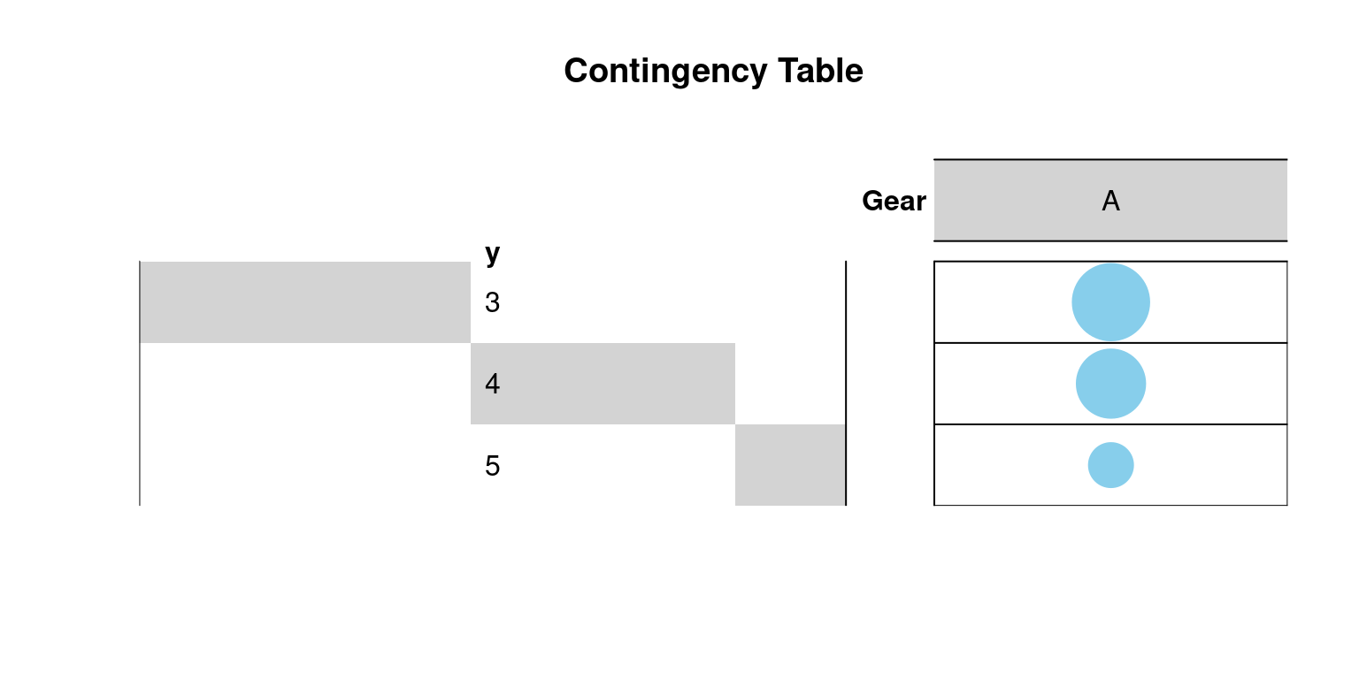
3. Calculation of Proportions
We calculate the proportions of cars in each gear category:
# Calculate proportions of cars in each gear category
gear_proportions <- prop.table(gear_counts)
gear_proportions
      3       4       5
0.46875 0.37500 0.15625
4. Running the Chi-Square Goodness-of-Fit Test
We specify the expected probabilities for each gear category and perform the chi-square goodness-of-fit test:
# Specify the expected probabilities for each gear category
expected_probs <- c(0.5,
                    0.3,
                    0.2)

# Perform the chi-square goodness-of-fit test using observed proportions and expected probabilities
chisq_test_result <- chisq.test(gear_proportions,
                                p=expected_probs)
chisq_test_result
    Chi-squared test for given probabilities

data:  gear_proportions
X-squared = 0.030273, df = 2, p-value = 0.985
5. Interpretation
After running the chi-square goodness-of-fit test using the provided expected probabilities, the output provides important information:
Chi-squared test for given probabilities: This line indicates that the test conducted is specifically a chi-square goodness-of-fit test. It’s designed to assess whether the observed data fits the expected probabilities we’ve provided.
data: gear_proportions: This line specifies the dataset used for the test, which is the gear_proportions dataset. This dataset contains the observed proportions of cars in different gear categories.
X-squared = 0.030273: This value represents the chi-square statistic (X²), which is a measure of how closely the observed proportions align with the expected probabilities. In this case, the calculated chi-square statistic is approximately 0.030273.
df = 2: This indicates the degrees of freedom (df) associated with the chi-square distribution. In a goodness-of-fit test like this one, the df is calculated as one less than the number of categories being analyzed. Here, since there are three gear categories (3, 4, and 5), df equals 2.
p-value = 0.985: The p-value is a crucial result of the test. It represents the probability of observing a chi-square statistic as extreme as the calculated value (0.030273) under the assumption that there is no significant difference between the observed and expected proportions. In this case, the high p-value of 0.985 suggests that the observed data aligns well with the expected probabilities. A high p-value implies that there is no strong evidence to reject the null hypothesis, which means that the data does not provide significant grounds to believe that the observed proportions are different from what was expected.
In summary, this output tells us that the chi-square goodness-of-fit test was conducted using the observed proportions of cars in different gear categories and the specified expected probabilities. The resulting high p-value (0.985) indicates that there is no strong reason to conclude that the observed proportions significantly differ from the expected probabilities, thus failing to reject the null hypothesis.
The Chi-Square Goodness of Fit test is employed to assess whether observed data conforms to an expected distribution, particularly when dealing with categorical data. It evaluates the similarity between observed and expected frequencies across different categories, typically through a chi-square statistic and follows a chi-square distribution.
It is used when you have categories or groups, and it helps determine if the observed data matches an expected distribution within those categories. It’s like checking if things are divided as you’d expect.
In contrast, the Z-test for Proportions focuses on comparing a sample proportion with a known population proportion, typically in binary data scenarios. It uses a Z-score to measure the difference and follows a standard normal distribution.
It helps us assess if the proportion of “yes” responses in our sample significantly differs from a known or expected proportion. It’s like comparing one group to a known standard.
The overall objective of this test is to qualitatively and quantitatively analyze and understand the interrelationships between different categorical variables in the mtcars dataset.
Specifically, in this illustration, the test aims to explore the association between the number of cylinders (cyl) and transmission type (am), in the dataset.
mtcars.This step ensures that R treats these variables as categorical data, which is necessary for a Chi-Square test.
data(mtcars)
mtcars$cyl <- as.factor(mtcars$cyl)
mtcars$am  <- as.factor(mtcars$am)
mtcars$gear <- as.factor(mtcars$gear)ctab <- table(mtcars$am,
mtcars$cyl)
ctab
     4  6  8
  0  3  4 12
  1  8  3  2
A contingency table (ctab) is created to summarize the relationship between two categorical variables.
The balloonplot function from the gplots library is used to visually represent the contingency table.
library("gplots")
# 1. convert the data as a table
dt <- as.table(
  as.matrix(ctab))

# 2. Graph
balloonplot(t(dt),
            main ="Contingency Table",
            xlab ="cyl", ylab="am",
            label = FALSE,
            show.margins = FALSE)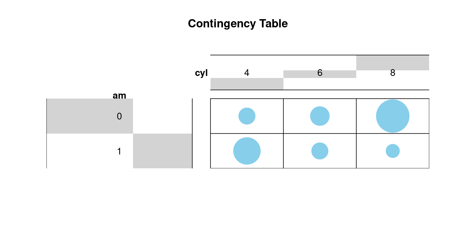
chisq.test() as follow:chisq <- chisq.test(ctab)Warning in chisq.test(ctab): Chi-squared approximation may be incorrectchisq
    Pearson's Chi-squared test

data:  ctab
X-squared = 8.7407, df = 2, p-value = 0.01265
In our example, the row and the column variables are statistically significantly associated (p-value = 0.01265). This indicates a statistically significant association between the variables at common alpha levels (like 0.05).
The observed and the expected counts can be extracted from the result of the test as follows:
# Observed counts
chisq$observed
     4  6  8
  0  3  4 12
  1  8  3  2
# Expected counts
round(chisq$expected, 2)
       4    6    8
  0 6.53 4.16 8.31
1 4.47 2.84 5.69Positive residuals are positive values in cells specify an attraction (positive association) between the corresponding row and column variables.
Negative residuals implies a repulsion (negative association) between the corresponding row and column variables.
round(chisq$residuals, 3)
         4      6      8
  0 -1.382 -0.077  1.279
  1  1.670  0.093 -1.546
The overall qualitative objective of running the Chi-Square Test of Independence, as described in the example using the mtcars dataset in R, is to determine whether there is a statistically significant relationship between different categorical variables in the dataset. Specifically, the test aims to explore the association between variables like the number of cylinders (cyl), transmission type (am), in the dataset. The key goals and insights sought from this test include:
Understanding Relationships Between Variables: To identify if there is a statistically significant association between different categorical variables in the dataset. For instance, it might reveal whether the type of transmission (automatic or manual) is associated with the number of cylinders or gears in the cars.
Testing Hypotheses About Associations: The Chi-Square Test of Independence is essentially a hypothesis test. The null hypothesis states that there is no association between the variables (they are independent), while the alternative hypothesis suggests there is an association (they are not independent).
Guiding Data-Driven Decisions: By understanding the relationships between variables, businesses, analysts, or data scientists can make informed decisions. For example, if a significant association is found between certain car features, it might influence marketing strategies or product development.
Visualizing Data Relationships: Through graphical representation like balloon plots, the test provides a visual understanding of the strength and nature of the relationships between categorical variables.
Quantitative Analysis of Associations: Beyond just identifying if an association exists, the test provides measures like the chi-square statistic, p-value, observed and expected counts, and Pearson residuals. These measures quantify the strength of association and help in understanding the nature of the relationship (whether it’s positive or negative).
The overall objective of this test is to qualitatively and quantitatively analyze and understand the interrelationships between different categorical variables in the mtcars dataset.
[1] Agresti, A. (2002). Categorical data analysis (2nd ed.). Wiley.
Hair Jr, J. F., Black, W. C., Babin, B. J., & Anderson, R. E. (2010). Multivariate data analysis: A global perspective (7th ed.). Pearson Education.
Everitt, B. S. (1992). The analysis of contingency tables (2nd ed.). Chapman and Hall.