Linear Regression.

Mar 23, 2024

Linear regression is a statistical method for determining the relationship between one or more independent variables and a dependent variable. It is a simple and powerful data modeling and analysis tool that can assist in making predictions or identifying trends.
The primary goal of linear regression is to identify the best-fitting line or plane that describes the relationship between the independent and dependent variables. The regression line or plane represents the predicted value of the dependent variable given a particular value of the independent variable.
Linear regression, in its most basic form, involves fitting a straight line to a set of data points. When there is only one independent variable, this is known as Simple Linear Regression. When there are two or more independent variables, it is known as Multiple Linear Regression.
Linear regression makes several data assumptions, including that the relationship between the independent and dependent variables is linear, the errors or residuals are normally distributed, and there is no multicollinearity (high correlation) among the independent variables.
Linear regression can be used for a variety of purposes, including forecasting sales, predicting future trends, and estimating the impact of various variables on a specific outcome. It is widely used in a variety of fields, including economics, marketing, finance and social sciences. [1]

Business Applications of Linear Regression

Marketing

Sales forecasting: Using historical data and other factors such as pricing, advertising, and promotional activities, linear regression can be used to forecast future sales. This can assist marketers in optimizing their marketing mix and increasing sales performance.
Customer segmentation: Linear regression can be used to analyze customer groups based on demographic, psychographic, and behavioral characteristics. Marketers can use this information to tailor their marketing messages and offerings to specific customer segments.
Product development: Linear regression can be used to characterize the product features and attributes that are most important to customers and then optimize the product design and development process accordingly.
Advertising effectiveness: Multiple linear regression can be used to measure the effectiveness of advertising campaigns and to identify the most effective advertising messages and media channels for reaching and persuading target customers. [2]

Finance

Portfolio management: Linear regression can be used to examine the relationship between various variables such as interest rates, inflation, and market volatility, as well as to optimize portfolio allocation and risk management strategies.
Credit scoring: Using Linear regression, credit scoring models can be created that predict the likelihood of default based on factors such as credit history, income, and employment status.
Asset pricing: Linear regression can be used to estimate the fair value of assets such as stocks, bonds, and options by analyzing the relationship between various factors such as earnings, dividends, and market trends.
Financial forecasting: Using historical data and other factors such as macroeconomic indicators and industry trends, Linear regression can be used to forecast financial outcomes such as revenue, earnings, and cash flow.
Risk management: Linear regression can be used to analyze the relationship between different risk factors, such as interest rates, exchange rates, and commodity prices, and to develop risk management strategies that reduce exposure to these risks. [3]

Organizational Behavior

Linear Regression can be used to investigate various aspects of organizational behavior, such as employee performance, workforce diversity, leadership effectiveness, organizational culture, and employee well-being.

Employee performance: Linear regression can be used to investigate the relationship between various factors like job satisfaction, motivation, and training and employee performance outcomes like productivity, job satisfaction, and turnover.
Workforce diversity: Linear regression can be used to examine the relationship between demographic diversity, cultural diversity, and social diversity and organizational outcomes such as creativity, innovation, and problem-solving.
Leadership effectiveness: Linear regression can be used to examine the relationship between various factors like leadership style, communication, and decision-making and leadership outcomes like employee motivation and job satisfaction.
Organizational culture: Linear regression can be used to investigate the relationship between organizational values, norms, and beliefs and organizational outcomes such as employee engagement, retention, and performance.
Employee well-being: Multiple linear regression can be used to examine the relationship between work-life balance, social support, and job demands and employee well-being outcomes such as stress, burnout, and health. [4]

Simple Linear Regression

Overview

Simple linear regression is used to model the relationship between a dependent variable and a single independent variable.
The goal of simple linear regression is to find the best fit line.
The best fit line is determined by minimizing the sum of the squared distances between the actual and predicted values of the dependent variable based on the independent variable.
The independent variable is plotted on the x-axis, and the dependent variable is plotted on the y-axis, to create a scatter plot and visualize the best fit line. [5]

Model of Simple Linear Regression

The model equation for a simple linear regression model is:

\[\begin{equation} \label{eq:slr} y = β_0 + β_1x + ε \end{equation}\]

$y$ is the dependent variable
$x$ is the independent variable
$β_0$ is the intercept (the value of $y$ when $x = 0$)
$β_1$ is the slope (the change in y for a one-unit change in x)
$ε$ is the error term (represents the random variability in the data)

The goal of the simple linear regression model shown in ($\ref{eq:slr}$), is to estimate the values of $β_0$ and $β_1$ given that minimize the sum of squared errors (SSE) between the observed values of $y$ and the predicted values of $y$.
There are several methods for estimating the values of $β_0$ and $β_1$, the most common of which is the called Ordinary Least Squares (OLS).
The Ordinary Least Squares (OLS) method calculates the values of

$β_0$ and $β_1$ that minimize the sum of squared errors (SSE) between the observed and predicted values of $y$.
After estimating the values of $β_0$ and $β_1$, the model can be used to predict the value of $y$, for any given value of $x$. [6]

Running Simple Linear Regression in R

Goal

Consider the mtcars data. Suppose we need to fit a simple linear regression model to predict mpg (miles per gallon) based on the predictor variable: wt (weight).
We would like to estimate it using Ordinary Least Squares.

Steps

# load mtcars dataset
data(mtcars)

# fit a simple linear regression model
model0 <- lm(mpg ~ wt, data = mtcars)

# print the model summary
summary(model0)


Call:
lm(formula = mpg ~ wt, data = mtcars)

Residuals:
    Min      1Q  Median      3Q     Max 
-4.5432 -2.3647 -0.1252  1.4096  6.8727 

Coefficients:
            Estimate Std. Error t value Pr(>|t|)    
(Intercept)  37.2851     1.8776  19.858  < 2e-16 ***
wt           -5.3445     0.5591  -9.559 1.29e-10 ***
---
Signif. codes:  0 '***' 0.001 '**' 0.01 '*' 0.05 '.' 0.1 ' ' 1

Residual standard error: 3.046 on 30 degrees of freedom
Multiple R-squared:  0.7528,    Adjusted R-squared:  0.7446 
F-statistic: 91.38 on 1 and 30 DF,  p-value: 1.294e-10

Using the lm() function in R, we can fit a simple linear regression model in which the dependent variable (mpg) is regressed on the independent variable (wt).
The data argument specifies the dataset, and mpg ~ wt specifies the linear regression model formula, where mpg is the dependent variable and wt is the independent variable.
The summary() function is called to print the model’s results. The output gives the estimated coefficients, standard errors, t-statistics, and p-values for each variable in the model, as well as the overall R-squared value and other statistics related to model fit.
Substituting the values of $\beta$ coefficients from the above regression output, we can write the model as follows.

\[\begin{equation} \label{eq:slr2} mpg = 37.2851 -5.3445 wt + ε \end{equation}\]

Visualizing Simple Linear Regression in R

Goal

Suppose we need to visualize the above simple linear regression model to predict mpg (miles per gallon) based on the predictor variable: wt (weight).
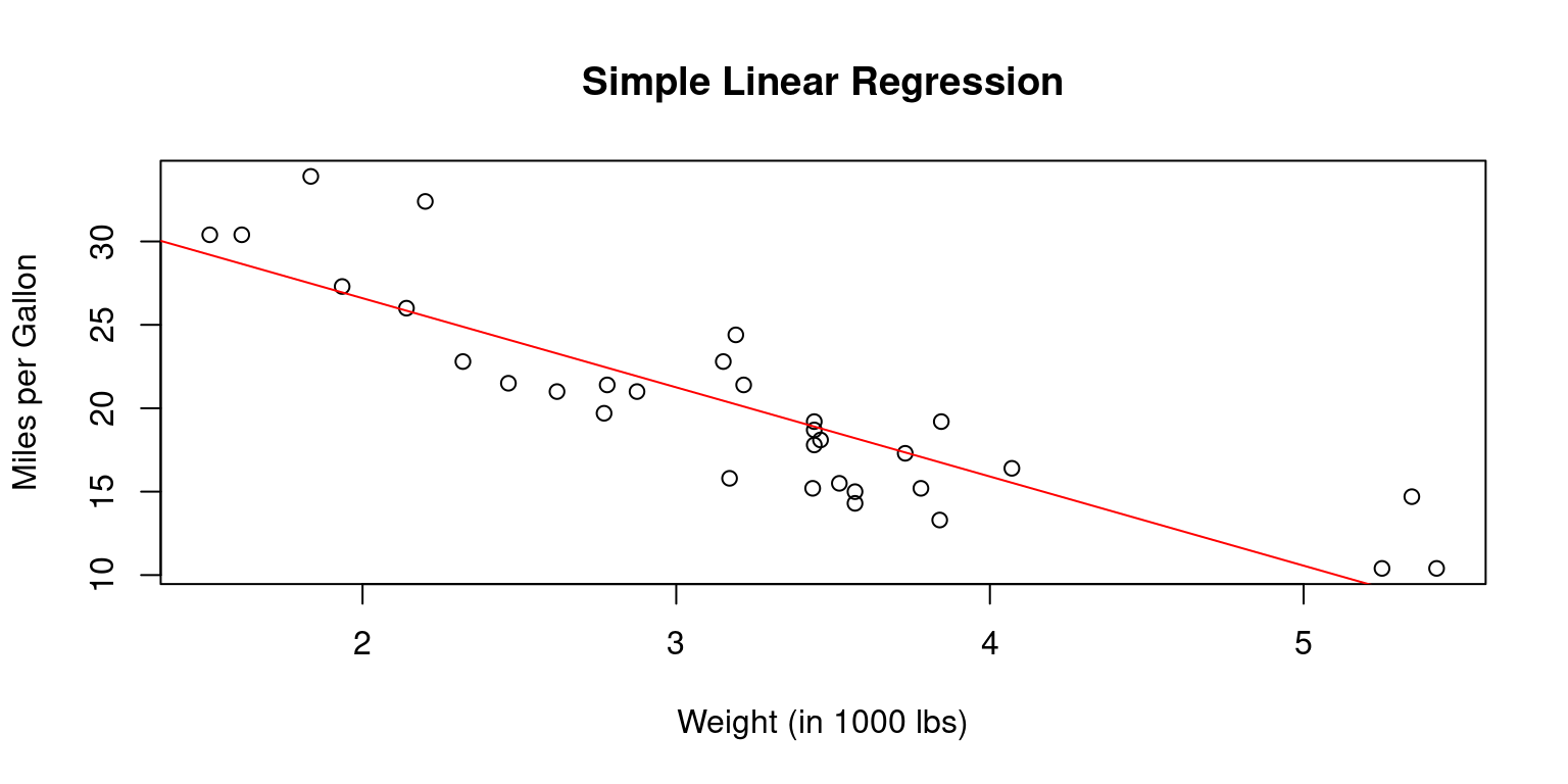
One way of doing this is to create a scatter plot.

Steps

# plot the data and the regression line
plot(mtcars$wt, 
     mtcars$mpg, 
     main = "Simple Linear Regression", 
     xlab = "Weight (in 1000 lbs)", 
     ylab = "Miles per Gallon")
abline(model0, col = "red")

We create a scatter plot of the data using the plot() function, where the x-axis represents the weight of the car in thousands of lbs, and the y-axis represents the miles per gallon.
We also use the main and xlab, ylab arguments to add a title and axes labels.
Finally, we use the abline() function to add the regression line to the plot, which takes the model object as an argument and plots the regression line. Using the col argument, we change the color of the line.
This code generates a scatter plot of the data with the regression line overlaid on top, allowing us to easily visualize the relationship between the dependent and independent variables. [7]

Multiple Linear Regression

Overview

Multiple linear regression is a statistical technique used to model the relationship between a dependent variable and multiple independent variables.
The goal of multiple linear regression is to find the linear equation that best explains the relationship between the dependent variable and the independent variables. [8]

Model of Multiple Linear Regression

The model equation for a multiple linear regression model with p independent variables is:

\[\begin{equation} \label{eq:mlr} y = β_0 + β_1x_1 + β_2x_2 + … + β_px_p + ε \end{equation}\]

$y$ is the dependent variable
$x_1$, $x_2$, …, $x_p$ are the independent variables
$β_0$ is the intercept (the value of $y$ when all independent variables are 0)
$β_1$, $β_2$, …, $β_p$ are the coefficients that represent the change in $y$ for a one-unit change in each independent variable, holding all other variables constant
$ε$ is the error term (represents the random variability in the data)

The model given in ($\ref{eq:mlr}$) is the most popular regression model.

Ordinary Least Squares (OLS) Estimation

Ordinary Least Squares (OLS) regression is the most widely used statistical estimation method for multiple linear regression.
OLS estimates the values of $β_0$, $β_1$, $β_2$, …, $β_p$ that minimize the sum of squared errors (SSE) between the observed values of $y$ and the predicted values of $y$.
Once the values of $β_0$, $β_1$, $β_2$, …, $β_p$ have been estimated, the model can be used to predict the value of $y$ for any given values of $x_1$, $x_2$, …, $x_p$. [8]

Running Multiple Linear Regression using OLS in R

Goal

Consider the mtcars data. Suppose we need to fit a multiple linear regression model to predict mpg (miles per gallon) based on the predictor variables: disp (displacement), hp (horsepower), and wt (weight) and cyl (number of cylinders).
We would like to estimate it using Ordinary Least Squares.

Steps

At the outset, we need to ensure that the data types are correct

# Load the mtcars dataset
data(mtcars)

# `cyl` (number of cylinders) needs to set as a factor
mtcars$cyl <- as.factor(mtcars$cyl)

# verify that `cyl` is a factor
str(mtcars$cyl)

 Factor w/ 3 levels "4","6","8": 2 2 1 2 3 2 3 1 1 2 ...

# verify that `mpg`, `disp`, `hp`, `wt` are numeric
str(mtcars$mpg)

 num [1:32] 21 21 22.8 21.4 18.7 18.1 14.3 24.4 22.8 19.2 ...

str(mtcars$disp)

 num [1:32] 160 160 108 258 360 ...

str(mtcars$hp)

 num [1:32] 110 110 93 110 175 105 245 62 95 123 ...

str(mtcars$wt)

 num [1:32] 2.62 2.88 2.32 3.21 3.44 ...

Now, we can run the multiple linear regression.

# Fit a multiple linear regression model
model <- lm(mpg ~ disp + hp + wt + cyl, 
            data = mtcars)

# View the summary of the model
summary(model)


Call:
lm(formula = mpg ~ disp + hp + wt + cyl, data = mtcars)

Residuals:
    Min      1Q  Median      3Q     Max 
-4.2740 -1.0349 -0.3831  0.9810  5.4192 

Coefficients:
             Estimate Std. Error t value Pr(>|t|)    
(Intercept) 36.002405   2.130726  16.897 1.54e-15 ***
disp         0.004199   0.012917   0.325  0.74774    
hp          -0.023517   0.012216  -1.925  0.06523 .  
wt          -3.428626   1.055455  -3.248  0.00319 ** 
cyl6        -3.466011   1.462979  -2.369  0.02554 *  
cyl8        -3.753227   2.813996  -1.334  0.19385    
---
Signif. codes:  0 '***' 0.001 '**' 0.01 '*' 0.05 '.' 0.1 ' ' 1

Residual standard error: 2.482 on 26 degrees of freedom
Multiple R-squared:  0.8578,    Adjusted R-squared:  0.8305 
F-statistic: 31.37 on 5 and 26 DF,  p-value: 3.18e-10

The lm() function is used to fit the model, and the data argument specifies the mtcars dataset.
The model formula specifies that mpg is the response variable and cyl, disp, hp, and wt are the predictor variables. The data argument specifies the dataset that the variables are taken from, which in this case is the mtcars dataset.
Recall that cyl is a categorical, factor variable that takes three levels $cyl = {4, 6, 8}$ corresponding to four, six and eight cylinder cars.
R sets the level $cyl = 4$ to be the base level by default. It creates two dummy variables cyl6 and cyl8 corresponding to six and eight cylinder cars. We have, cyl6=1 for six cylinder cars, cyl6=0 otherwise. We have, cyl8=1 for eight cylinder cars, cyl8=0 otherwise.
The beta coefficient estimate for cyl6 represents the expected difference in mpg between cars with six cylinders and cars with four cylinders.
The equation for the multiple linear regression model to predict mpg (miles per gallon) based on the predictor variables: disp (displacement), hp (horsepower), and wt (weight) and cyl (number of cylinders) is given as follows:

\[\begin{equation} \label{eq:mlr2} mpg = 36.0024 + 0.0042disp - 0.0235hp - 3.4286 wt - 3.4660 cyl_6 - 3.7532 cyl_8 + ε \end{equation}\]

The summary() function is used to view a summary of the model, which includes information such as the coefficients for each predictor variable, the standard errors, t-values, and p-values for each coefficient, the R-squared value, and more. This summary output can be used to interpret the results of the multiple linear regression model. [9]

Output of Multiple Linear Regression using OLS in R

Beta Coefficients Estimates

The beta coefficient estimate for a predictor variable represents the change in the response variable that is associated with a one-unit increase in that predictor variable, while holding all other predictor variables constant. In other words, it represents the effect that each predictor variable has on the response variable, after controlling for the effects of all other predictor variables in the model.
In the output of the multiple linear regression model, the “Coefficients” table shows the estimates of the beta coefficients (also known as regression coefficients or slope coefficients) for each predictor variable in the model. [9]
We can use the following code to extract the beta coefficients.

betas = model$coefficients
round(betas,4)

(Intercept)        disp          hp          wt        cyl6        cyl8 
    36.0024      0.0042     -0.0235     -3.4286     -3.4660     -3.7532

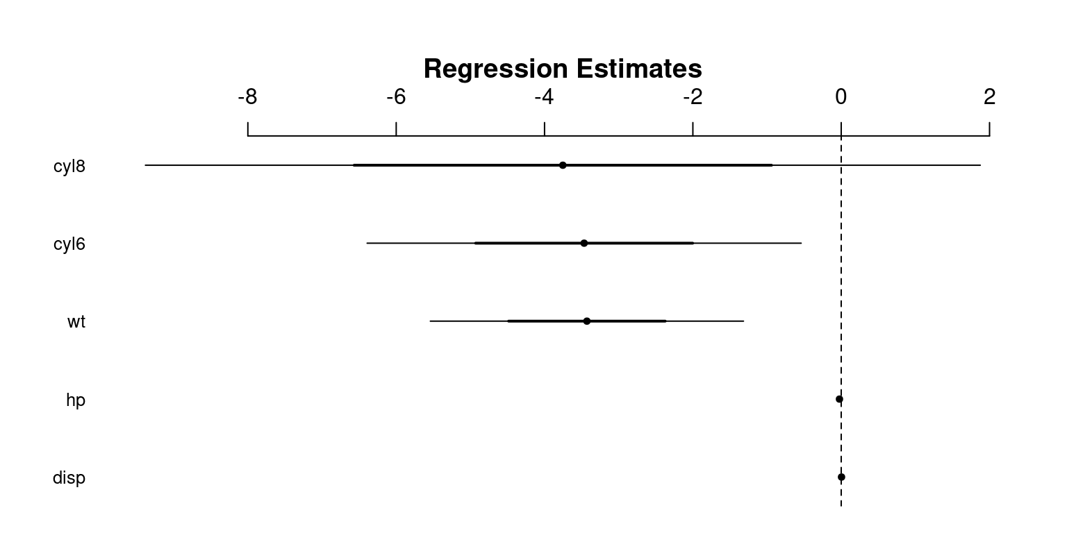
We can also visualize the beta coefficients. We use coefplot() in the arm package to plot the coefficients and their 95% credible intervals.

# Load the arm package
library(arm)

Loading required package: MASS

Loading required package: Matrix

Loading required package: lme4


arm (Version 1.13-1, built: 2022-8-25)

Working directory is /cloud/project

# Use coefplot() to plot the coefficients of the model
coefplot(model)

Interpretation of beta coefficient estimates [9]

Example 1:

The beta coefficient estimate for disp represents the estimated change in the “mpg” response variable associated with a one-unit increase in the disp predictor variable, while holding all other predictors constant.
The beta coefficient estimate for disp is 0.004199. This means that, on average, as the disp variable (engine displacement, in cubic inches) increases by one unit, the predicted mpg value for the car increases by 0.004199 units, while holding all other predictor variables constant.
However, as the p-value for disp is greater than the chosen threshold of 0.05, there is no evidence to suggest that this change is statistically significant at the 5% level, after controlling for the effects of the other predictor variables in the model. Therefore, it may not be appropriate to make any conclusive statements about the relationship between disp and mpg based solely on the beta coefficient estimate for disp in this model.

Example 2:

The the beta coefficient estimate for wt represents the estimated change in the mpg response variable associated with a one-unit increase in the wt predictor variable, while holding all other predictors constant.
The beta coefficient estimate for wt is -3.428626. This means that, on average, as the wt variable (weight of the car in thousands of pounds) increases by one unit, the predicted mpg value for the car decreases by 3.428626 units, while holding all other predictor variables constant.

Example 3:

The beta coefficient estimate for cyl6 is -3.466011. This means that, on average, cars with six cylinders have a predicted “mpg” value that is 3.466011 lower than cars with four cylinders, after accounting for the effects of the other predictor variables in the model.
Similarly, the beta coefficient estimate for cyl8 is -3.753227. This means that, on average, cars with eight cylinders have a predicted mpg value that is 3.753227 lower than cars with four cylinders, after accounting for the effects of the other predictor variables in the model.

Standard Errors

In multiple linear regression, the standard error is a measure of the variability of the estimated coefficients of the predictor variables in the model.
It reflects the variability of the estimated coefficients due to the random error in the data. It represents the average amount that the estimated coefficients would vary if we fit the same model to different samples of data from the population.
The standard error is estimated from the residual standard error of the model, which is a measure of the variability of the residuals or the differences between the predicted and observed values of the response variable.
A smaller standard error means a more precise estimate of the coefficient, and more likely to accurately reflect the true relationship between the independent variable and the dependent variable. [9]

Example 1:

In the output of the linear regression model, “Std. Error” of wt refers to the standard error of the estimate for the coefficient of the independent variable wt (weight of the car).
The “Std. Error” of wt is given as 1.0554. This means that the estimated coefficient for wt is expected to vary by about 1.0554 units across different samples of data that could have been collected. [9]

t-values and p-values

The t-value measures the number of standard errors the estimated coefficient is away from zero. It is calculated by dividing the estimated coefficient by its standard error.
A higher absolute t-value suggests that the estimated coefficient is more significant and more likely to accurately reflect the true relationship between the independent variable and the dependent variable.
It’s important to note that the t-value is used to calculate the p-value for the coefficient estimate. A small p-value indicates that the coefficient is statistically significant and not likely to have occurred by chance.
The p-value is the probability of observing a t-value as extreme or more extreme than the observed t-value, assuming that the true coefficient is zero.
A small p-value indicates that it is unlikely that the observed t-value occurred by chance, and suggests that the true coefficient is not zero (i.e., there is a statistically significant relationship between wt and mpg). [9]

Example 1:

In the output, the “t-value” of wt is given as -3.248. This means that the estimated coefficient for wt is -3.248 standard errors away from zero.
A negative t-value indicates that there is an inverse relationship between the independent variable and the dependent variable. Since the t-value is relatively large (in absolute value) and negative, it suggests that the estimated coefficient for wt is statistically significant and has a significant impact on the dependent variable (mpg).
In this case, the p-value for wt is 0.00319, indicating that the estimated coefficient for wt is statistically significant and has a significant impact on the dependent variable.
In the output, the “t-value” of wt is -3.248, and the degrees of freedom for the t-distribution is 26 (which is the sample size minus the number of parameters estimated in the model).

[9]

Interpretation of p-value, Pr(>|t|)

Example 2:

In the output, the beta coefficient estimate for disp is 0.004199 with a standard error of 0.012917, a t-value of 0.325, and a p-value of 0.74774.
The p-value for disp is greater than the chosen threshold of 0.05, indicating that the beta coefficient estimate for “disp” is not statistically significant at the 5% level. This means that, after controlling for the effects of the other predictor variables in the model, there is no evidence to suggest that the disp variable has a significant linear relationship with the mpg response variable.
Therefore, the disp variable is not a significant predictor of the mpg response variable in the model. [9]

Example 3:

In the output, the beta coefficient estimate for wt is -3.428626 with a standard error of 1.055455, a t-value of -4.223, and a p-value of 0.0002.
The p-value for wt is less than the chosen threshold of 0.05, indicating that the beta coefficient estimate for wt is statistically significant at the 5% level.
This means that, after controlling for the effects of the other predictor variables in the model, there is evidence to suggest that the wt variable has a significant linear relationship with the mpg response variable. [9]

Example 4:

In the output, the beta coefficient estimate for cyl_6 is -3.466011 with a standard error of 1.462979, a t-value of -2.369, and a p-value of 0.02554. Similarly, the beta coefficient estimate for cyl_8 is -3.753227 with a standard error of 2.813996, a t-value of -1.334, and a p-value of 0.19385.
The p-value for cyl_6 is greater than the chosen threshold of 0.05, indicating that the beta coefficient estimate for cyl_6 is not statistically significant at the 5% level.
This means that, after controlling for the effects of the other predictor variables in the model, there is no evidence to suggest that the average mpg for cars with six cylinders is significantly different from that for cars with four cylinders.
On the other hand, the p-value for cyl_8 is less than 0.05, indicating that the beta coefficient estimate for cyl_8 is statistically significant at the 5% level.
This means that, after controlling for the effects of the other predictor variables in the model, there is evidence to suggest that the average mpg for cars with eight cylinders is significantly different from that for cars with four cylinders.
Also, the negative beta coefficient estimate for cyl_8 indicates that, on average, cars with eight cylinders have a lower predicted mpg value than cars with four cylinders, while holding all other predictor variables constant. [9]

Confidence Intervals

In multiple linear regression, the confidence interval can be interpreted as a range of values that we are x% confident contains the true population coefficient, where x is the chosen level of confidence.
The most common level of confidence is 95%, but other levels of confidence, such as 90% or 99%, can also be used.
The confidence interval is based on the standard error and the t-distribution, which takes into account the sample size and the degrees of freedom of the model.
In the output of the linear regression model, we can calculate the confidence interval for the beta coefficient of wt (weight of the car) at a desired confidence level (e.g., 95%) using the t-distribution.
The following code will output the confidence intervals

# View the 95% confidence intervals of the estimated coefficients
confint(model, level = 0.95)

                  2.5 %       97.5 %
(Intercept) 31.62263411 40.382174889
disp        -0.02235276  0.030750496
hp          -0.04862749  0.001594483
wt          -5.59814537 -1.259106203
cyl6        -6.47320809 -0.458813851
cyl8        -9.53747788  2.031023933

In the output, the confidence intervals of the estimated coefficients are displayed in a table with two columns, “2.5 %” and “97.5 %”.
For example, the confidence interval for the estimated coefficient of wt is (-5.985, -1.617), which means that we are 95% confident that the true population coefficient for wt lies within this range.
If the confidence interval for a coefficient does not include 0, we can conclude that the corresponding predictor variable is likely to be a significant predictor of the response variable at the 5% level of significance.
The formula for the confidence interval in multiple linear regression is: $CI = \beta ± t * SE$, where $t” represents the t-value and $SE$ represents the Standard Error.

the coefficient estimate is the point estimate of the coefficient,
the t-value is the critical value from the t-distribution with $n-p-1$ degrees of freedom, where
$n$ is the sample size and $p$ is the number of predictor variables in the model,
the standard error $SE$ is a measure of the variability of the estimated coefficient
The critical value from the t-distribution depends on the level of confidence and the degrees of freedom. For example, for a 95% confidence interval with 25 observations and 3 predictor variables, the critical value is approximately 2.306. [10]

Visualizing Multiple Linear Regression in R

Goal

Suppose we need to visualize the above multiple linear regression model to predict mpg (miles per gallon) based on multiple predictor variables.
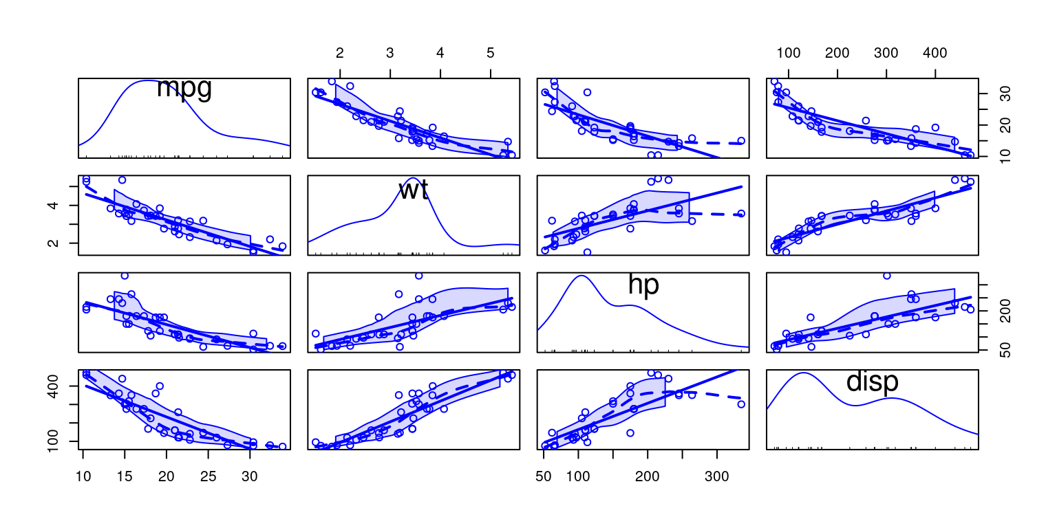
There is no good way of doing this. One limited way of doing this is to create a scatter plot matrix.

Steps

# Create a scatterplot matrix of the variables
library(car)

Loading required package: carData


Attaching package: 'car'

The following object is masked from 'package:arm':

    logit

scatterplotMatrix(~mpg + wt + hp + disp, 
                  data = mtcars)

# Add the regression line to the scatterplot matrix
abline(model, col = "blue")

Warning in abline(model, col = "blue"): only using the first two of 6
regression coefficients

This code will create a scatterplot matrix of the variables (mpg, wt, hp, disp) in the mtcars data set, and will add a regression line to the plot to visualize the relationship between mpg, wt, hp,`disp.
The scatterplot matrix will show the scatterplots of all three variables, and the regression line will show the predicted relationship between mpg, wt, hp, disp.
Note that we will need to have the car package installed in order to create the scatterplot matrix. If we don’t have the package installed, we can install it by running install.packages("car").

Residuals and Residual Standard Error

Residuals

In the output of the linear regression model, “Residuals” refer to the differences between the predicted values of the dependent variable (mpg) and the actual observed values of the dependent variable in the dataset (mtcars).
The residuals are important to examine because they can provide information about the accuracy of the model. Ideally, the residuals should be normally distributed around zero, indicating that the model is accurately predicting the values of the dependent variable. If the residuals are not normally distributed or have a pattern, this could indicate that the model is not accurately predicting the values of the dependent variable and may require further refinement.
In the above example, the residuals are the differences between the predicted values and actual values of the dependent variable cyl, which cannot be explained by the independent variables (cyl, disp, hp, and wt) included in the model.
Analyzing the residuals can help us check whether the assumptions of the multiple linear regression model are met, and can also help us identify outliers or influential observations that may be affecting the model fit.

# Review the Residuals
summary(model)


Call:
lm(formula = mpg ~ disp + hp + wt + cyl, data = mtcars)

Residuals:
    Min      1Q  Median      3Q     Max 
-4.2740 -1.0349 -0.3831  0.9810  5.4192 

Coefficients:
             Estimate Std. Error t value Pr(>|t|)    
(Intercept) 36.002405   2.130726  16.897 1.54e-15 ***
disp         0.004199   0.012917   0.325  0.74774    
hp          -0.023517   0.012216  -1.925  0.06523 .  
wt          -3.428626   1.055455  -3.248  0.00319 ** 
cyl6        -3.466011   1.462979  -2.369  0.02554 *  
cyl8        -3.753227   2.813996  -1.334  0.19385    
---
Signif. codes:  0 '***' 0.001 '**' 0.01 '*' 0.05 '.' 0.1 ' ' 1

Residual standard error: 2.482 on 26 degrees of freedom
Multiple R-squared:  0.8578,    Adjusted R-squared:  0.8305 
F-statistic: 31.37 on 5 and 26 DF,  p-value: 3.18e-10

In the output, the “Residuals” section includes information about the minimum and maximum residuals, as well as the first and third quartiles, the median of the residuals. This information can be used to assess the distribution and potential patterns in the residuals.
To extract the residuals from a multiple linear regression model in R, we can use the resid() function on the model object.

# Extract the residuals
residuals <- resid(model)

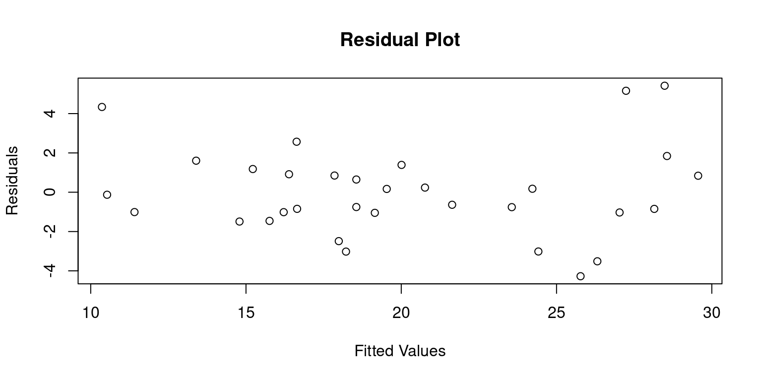
We can also create a scatter plot of the residuals against the fitted values (predicted values) to visually inspect whether the assumptions of the model are met:

# Plot the residuals against the fitted values
plot(fitted(model), residuals,
     xlab = "Fitted Values",
     ylab = "Residuals",
     main = "Residual Plot")

This will create a scatter plot of the residuals against the fitted values In this plot, we want to see a random scatter of points around the horizontal zero line, indicating that the residuals have a mean of zero and are evenly distributed across the range of fitted values.
If we see any patterns or trends in the residuals, such as a curved shape or a U-shape, this may indicate that the assumptions of the multiple linear regression model are not met and that the model may need to be modified or improved.
We can also calculate summary statistics for the residuals, such as the mean, standard deviation, and range, using the summary() function on the residuals object.

summary(residuals)

   Min. 1st Qu.  Median    Mean 3rd Qu.    Max. 
-4.2740 -1.0349 -0.3831  0.0000  0.9810  5.4192

\[11\]

Residual Standard Error

In the output of the linear regression model, “Residual standard error” refers to the standard deviation of the residuals.
It indicates how much the predicted values of the dependent variable deviate from the actual observed values, on average.
A lower residual standard error indicates that the model is better at predicting the values of the dependent variable.
The residual standard error provides a measure of the amount of variation in the dependent variable (mpg) that is not explained by the independent variables (cyl, disp, hp, and wt) included in the model.
In R, we can extract the RSE from a multiple linear regression model using the summary() function on the model object.

# Extract the RSE
rse <- summary(model)$sigma
rse

[1] 2.481678

In the output, the “Residual standard error” value is given as 2.639. This means that, on average, the predicted values of mpg deviate from the actual observed values by about 2.639 units.
It’s important to note that the residual standard error should be considered in the context of the range of values of the dependent variable. In this case, since the range of mpg values in the mtcars dataset is 10.4 to 33.9, a residual standard error of 2.639 might be considered reasonable, indicating that the model is making relatively accurate predictions of the dependent variable. [11]

Model Fit in Multiple Linear Regression

The model fit in multiple linear regression refers to how well the regression model fits the observed data. There are several measures of model fit that can be used to evaluate the performance of a multiple linear regression model.
R-squared: One commonly used measure of model fit is the R-squared value, which represents the proportion of the total variability in the response variable that is explained by the predictor variables in the model.

R-squared is a statistical measure that represents the proportion of variance in the dependent variable that can be explained by the independent variables in the model.
R-squared is sometimes called the coefficient of determination or the goodness-of-fit measure.
R-squared ranges from 0 to 1, with higher values indicating that the model explains a greater proportion of the variance in the dependent variable.
An R-squared of 0 indicates that the model does not explain any of the variance in the dependent variable, while an R-squared of 1 indicates that the model perfectly explains all of the variance in the dependent variable.
However, it is important to note that a high R-squared does not necessarily mean that the model is a good fit for the data or that it will be a good predictor. For example, an overfitted model that includes too many predictor variables may have a high R-squared, but it may not generalize well to new data.
Additionally, an R-squared of 0 does not necessarily mean that the model is not useful, as it may still provide some insight into the relationships between the variables in the model.

Adjusted R-squared:

The adjusted R-squared is a statistical measure of fit that accounts for the number of predictor variables included in the model.
Recall that the R-squared indicates the proportion of variation in the dependent variable (the variable we are trying to predict) that can be explained by the independent variables (the predictors) in the model.
However, as we add more variables to the model, the R-squared value will typically increase, even if the added variables do not actually improve the model’s ability to predict the dependent variable.
To address this issue, the “Adjusted R-squared” statistic adjusts for the number of predictor variables in the model. It penalizes models that include more variables that do not improve the model’s ability to predict the dependent variable.
The adjusted R-squared is calculated using the following formula: $AdjRSquared = 1 - [(1 - RSquared) * (n - 1) / (n - k - 1)]$, where $n$ is the sample size and $k$ is the number of predictor variables in the model.
The Adjusted R-squared will always be lower than the R-squared, since it adjusts for the number of predictor variables.
A higher Adjusted R-squared value indicates that the model is a better fit for the data, as it indicates that more of the variation in the dependent variable is being explained by the independent variables, and not just due to chance or noise.

F-statistic:

In linear regression, the F-statistic is a statistical measure that is used to test the overall significance of the model.
It measures the ratio of the explained variance to the unexplained variance in the dependent variable.
It is calculated by dividing the mean square for the model by the mean square for the residuals.
The F-statistic is based on the null hypothesis that all of the coefficients in the model are equal to zero, indicating that the independent variables do not have any effect on the dependent variable.
The alternative hypothesis is that at least one of the coefficients in the model is not equal to zero, indicating that the independent variables do have an effect on the dependent variable.
If the F-statistic is large and the associated p-value is small, this provides evidence against the null hypothesis and suggests that the model is a good fit for the data.
However, if the F-statistic is small and the associated p-value is large, this suggests that the model is not a good fit for the data, and that the null hypothesis cannot be rejected.
It is important to note that while the F-statistic tests the overall significance of the model, it does not provide information about the individual significance of the coefficients or the relative importance of the predictor variables.

Calculating R-squared, Adjusted R-squared, F-statistic in R

We can read the R-squared, Adjusted R-squared, F-statistic from the output of the summary() function.

# Display the model summary
summary(model)


Call:
lm(formula = mpg ~ disp + hp + wt + cyl, data = mtcars)

Residuals:
    Min      1Q  Median      3Q     Max 
-4.2740 -1.0349 -0.3831  0.9810  5.4192 

Coefficients:
             Estimate Std. Error t value Pr(>|t|)    
(Intercept) 36.002405   2.130726  16.897 1.54e-15 ***
disp         0.004199   0.012917   0.325  0.74774    
hp          -0.023517   0.012216  -1.925  0.06523 .  
wt          -3.428626   1.055455  -3.248  0.00319 ** 
cyl6        -3.466011   1.462979  -2.369  0.02554 *  
cyl8        -3.753227   2.813996  -1.334  0.19385    
---
Signif. codes:  0 '***' 0.001 '**' 0.01 '*' 0.05 '.' 0.1 ' ' 1

Residual standard error: 2.482 on 26 degrees of freedom
Multiple R-squared:  0.8578,    Adjusted R-squared:  0.8305 
F-statistic: 31.37 on 5 and 26 DF,  p-value: 3.18e-10

Alternately, we can also extract the R-squared, Adjusted R-squared, F-statistic, as follows.

# Extract the R-squared
r_squared <- summary(model)$r.squared

# Extract the adjusted R-squared
adj_r_squared <- summary(model)$adj.r.squared

# Print the adjusted R-squared
cat("R-squared:", r_squared, "\n")

R-squared: 0.8577974

cat("Adjusted R-squared:", adj_r_squared, "\n")

Adjusted R-squared: 0.8304507

# Extract the F-statistic and its associated p-value
f_statistic <- summary(model)$fstatistic[1]

# Print the F-statistic and its associated p-value
cat("F-statistic:", f_statistic, "\n")

F-statistic: 31.36754

Model Prediction in Multiple Linear Regression

In multiple linear regression, model prediction refers to the process of using the model to make predictions about the value of the dependent variable based on the values of the independent variables.
To make a prediction using a multiple linear regression model, we first need to specify the values of the independent variables for the observation we want to predict the dependent variable for.
Then, we use the coefficients estimated by the model to calculate the predicted value of the dependent variable.
Recall that the multiple linear regression equation can be written as: $y = β_0 + β_1x_1 + β_2x_2 + … + β_px_p + ε$, where $y$ is the dependent variable, $x_1$, $x_2$, …, $x_p$ are the independent variables, $β_0$ is the intercept, and $β_1$, $β_2$, …, $β_p$ are the coefficients for the independent variables. $ε$ represents the error term or residual, which represents the difference between the predicted value of $y$ and the actual value of $y$.
To make a prediction using this equation, we would substitute the values of $x_1$, $x_2$, …, $x_p$ into the equation and calculate the predicted value of $y$.

Prediction in Multiple Linear Regression in R

In R, we can make predictions using the fitted multiple linear regression model. For reference, let us summarize the model, we will be using for prediction.

# View the model summary to assess its performance and significance
summary(model)


Call:
lm(formula = mpg ~ disp + hp + wt + cyl, data = mtcars)

Residuals:
    Min      1Q  Median      3Q     Max 
-4.2740 -1.0349 -0.3831  0.9810  5.4192 

Coefficients:
             Estimate Std. Error t value Pr(>|t|)    
(Intercept) 36.002405   2.130726  16.897 1.54e-15 ***
disp         0.004199   0.012917   0.325  0.74774    
hp          -0.023517   0.012216  -1.925  0.06523 .  
wt          -3.428626   1.055455  -3.248  0.00319 ** 
cyl6        -3.466011   1.462979  -2.369  0.02554 *  
cyl8        -3.753227   2.813996  -1.334  0.19385    
---
Signif. codes:  0 '***' 0.001 '**' 0.01 '*' 0.05 '.' 0.1 ' ' 1

Residual standard error: 2.482 on 26 degrees of freedom
Multiple R-squared:  0.8578,    Adjusted R-squared:  0.8305 
F-statistic: 31.37 on 5 and 26 DF,  p-value: 3.18e-10

We will create a new dataframe for the data to be used for the prediction. And then, we will run the predict() function.

# Make predictions for a new car with weight of 2.5, 
# displacement of 200, horsepower of 100, six cylinders
new_car <- data.frame(wt = 2.5, disp = 200, hp = 100, cyl = 6)

# Convert cyl to a factor variable in the new data frame
new_car$cyl <- as.factor(new_car$cyl)

# Make the prediction based on the model using the predict() function
predict(model, newdata = new_car)

       1 
22.45295

In this example, we use summary() to review a multiple linear regression model. This model was estimated using the lm() function, with mpg as the dependent variable and wt, disp, hp, cyl as the independent variables.
The newdata argument specifies a data frame containing the values of the independent variables for a new car having weight of 2.5, displacement of 200, horsepower of 100, and 6 cylinders,
The output of the predict() function informs us that the predicted value of mpg for the new car, based on the fitted model, is 22.45295 mpg.

6 Assumptions made in Ordinary Least Squares (OLS) estimation

OLS estimation makes several assumptions, and violating these assumptions can lead to biased or inefficient estimates of the regression coefficients. The following are the assumptions of OLS regression:

1. Linearity:

The relationship between the dependent variable and independent variables is linear. This means that the effect of a change in an independent variable on the dependent variable is constant.

2. Independence:

The observations in the dataset are independent of each other. In other words, the value of one observation does not depend on the value of another observation.

3. Homoscedasticity:

The variance of the error terms is constant across all values of the independent variables. This assumption is also known as the assumption of constant variance.

4. Normality:

The error terms are normally distributed with a mean of zero. This means that the distribution of the errors is symmetric and bell-shaped.

5. No multicollinearity:

There is no perfect linear relationship among the independent variables. In other words, the independent variables are not highly correlated with each other.

6. No outliers:

There are no extreme observations that are far away from the general pattern of the data. Such outliers can have a large effect on the estimates of the regression coefficients.

It is important to check for these assumptions before using OLS regression, and there are various methods to test for them. If any of these assumptions are violated, alternative methods such as robust regression or non-parametric regression may be more appropriate. [8]

Quadratic Regression

Overview

Quadratic regression is a form of multiple regression where the relationship between the independent variable (x) and the dependent variable (y) is modeled as a quadratic function. This type of regression is used when the data suggests a parabolic relationship between the variables, meaning the trend in the data increases or decreases at a non-constant rate.

The quadratic regression equation can be represented as:

\[\begin{equation} y = \beta_0 + \beta_1x + \beta_2x^2 + \epsilon \end{equation}\]

where:

$y$ is the dependent variable,

$x$ is the independent variable,

$\beta_0$ is the intercept of the model,

$\beta_1$ is the coefficient for the linear term,

$\beta_2$ is the coefficient for the quadratic term, and

$\epsilon$ is the error term of the model.

The coefficients $\beta_0$, $\beta_1$, and $\beta_2$ are estimated through the regression analysis, aiming to fit the model such that it minimizes the sum of the squared differences between the observed and predicted values.

Applying Quadratic Regression in R with the `mtcars` dataset

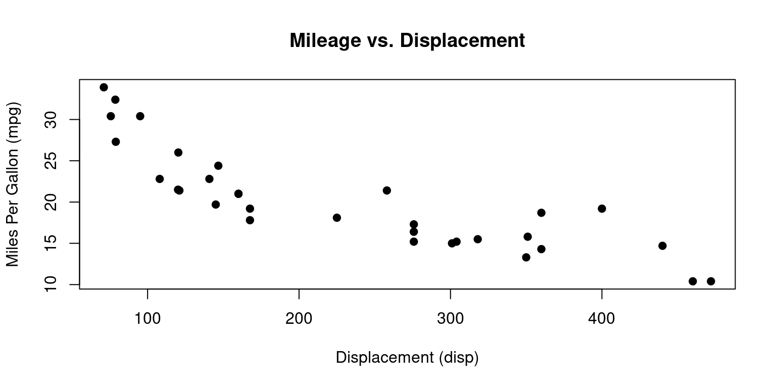
Let’s say we want to explore how the miles per gallon (mpg) of cars in the mtcars dataset is related to the displacement (disp), which is the engine size. We hypothesize that there’s a quadratic relationship between displacement and mpg.

Here’s a step-by-step guide on how to perform this analysis in R:

Visualize the Data: Plot disp versus mpg to visually inspect the relationship.
Fit the Quadratic Model: Use the lm() function to fit a quadratic regression model. We’ll include both the linear and quadratic terms of disp in the model.
Analyze the Results: Summarize the model to interpret the coefficients and assess the fit.

Step 1: Visualize the Data

plot(mtcars$disp, 
     mtcars$mpg, 
     main="Mileage vs. Displacement", 
     xlab="Displacement (disp)", 
     ylab="Miles Per Gallon (mpg)", 
     pch=19)

Step 2: Fit the Quadratic Model

The lm() function in R is used to fit a quadratic regression model by including both the linear and quadratic terms of displacement.

# Fit the quadratic regression model
model <- lm(mpg ~ disp + I(disp^2), 
            data=mtcars)

# Summarize the model to view coefficients and statistics
summary(model)


Call:
lm(formula = mpg ~ disp + I(disp^2), data = mtcars)

Residuals:
    Min      1Q  Median      3Q     Max 
-3.9112 -1.5269 -0.3124  1.3489  5.3946 

Coefficients:
              Estimate Std. Error t value Pr(>|t|)    
(Intercept)  3.583e+01  2.209e+00  16.221 4.39e-16 ***
disp        -1.053e-01  2.028e-02  -5.192 1.49e-05 ***
I(disp^2)    1.255e-04  3.891e-05   3.226   0.0031 ** 
---
Signif. codes:  0 '***' 0.001 '**' 0.01 '*' 0.05 '.' 0.1 ' ' 1

Residual standard error: 2.837 on 29 degrees of freedom
Multiple R-squared:  0.7927,    Adjusted R-squared:  0.7784 
F-statistic: 55.46 on 2 and 29 DF,  p-value: 1.229e-10

I(disp^2): The term I(disp^2) within the lm function call in R signifies the inclusion of a quadratic term for the variable disp (engine displacement) in the regression model. The I() function in R is used to indicate that disp^2 should be treated as a mathematical operation inside the formula. Without I(), the ^ symbol could be misinterpreted by the formula interface. In this context, I() ensures that disp is squared, and this squared term is then used as a predictor in the model.

Step 3: Analysis

Here’s how we can write the resulting quadratic model:

\[ \text{mpg} = 35.83 - 0.1053 \times \text{disp} + 0.0001255 \times \text{disp}^2 + \epsilon \]

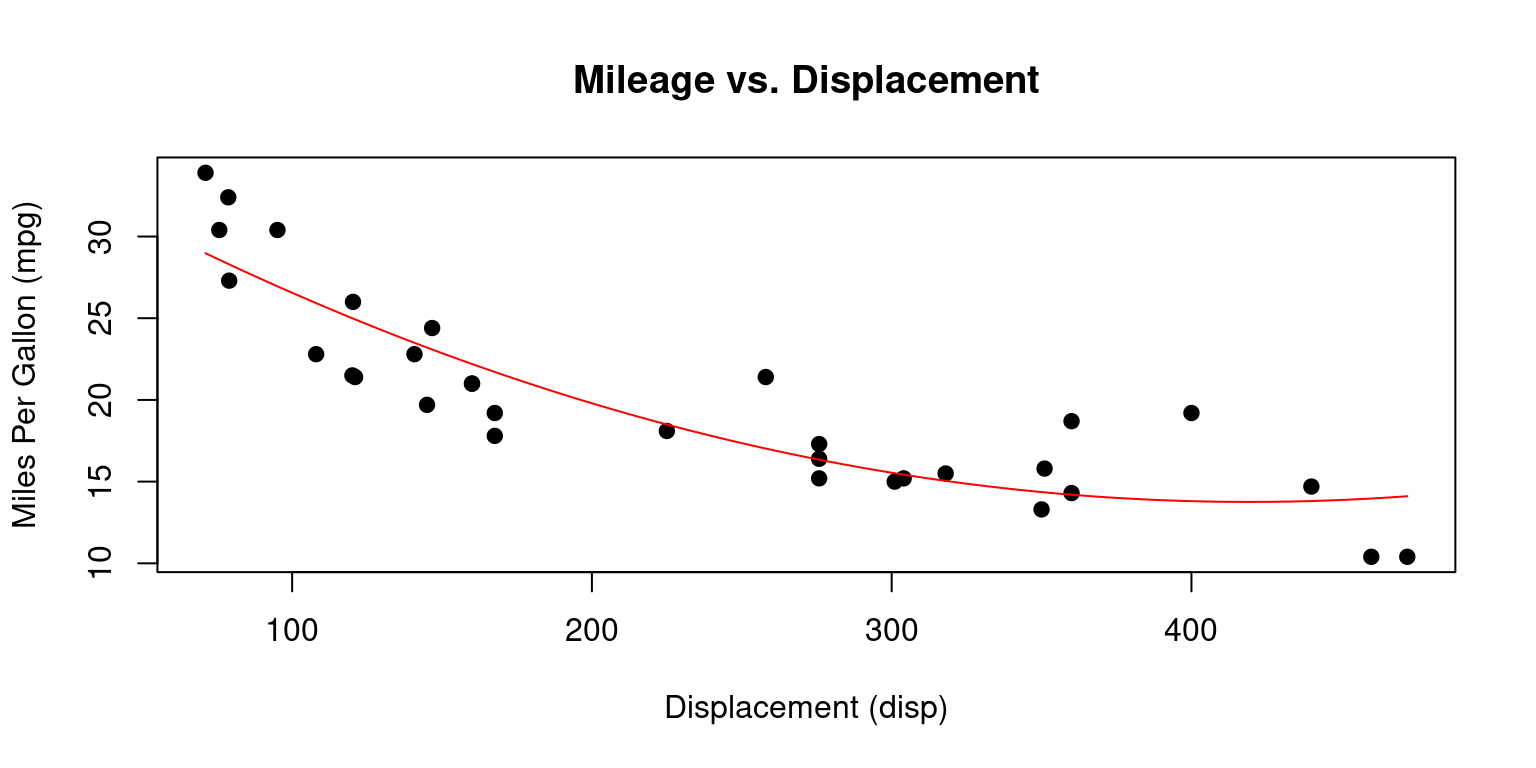
Here is how we can visualize it.

# Initial plot
plot(mtcars$disp, 
     mtcars$mpg, 
     main="Mileage vs. Displacement", 
     xlab="Displacement (disp)", 
     ylab="Miles Per Gallon (mpg)", 
     pch=19)

# Fit a quadratic regression model
model <- lm(mpg ~ disp + I(disp^2), 
            data=mtcars)

# Add the quadratic curve to the plot
# The curve expression uses the coefficients from the model
curve(coef(model)[1] + 
        coef(model)[2]*x + 
        coef(model)[3]*x^2, 
      add = TRUE, 
      col = "red", 
      from=min(mtcars$disp), to=max(mtcars$disp))

Coefficient for disp:

Estimate: The estimate of (-0.1053) indicates the effect of the linear term of displacement (disp) on miles per gallon (mpg). Specifically, for each one-unit increase in disp, mpg is expected to decrease by 0.1053 units, holding the effect of disp^2 constant. This suggests a negative linear relationship between engine displacement and fuel efficiency.
Std. Error: The standard error of the estimate is (0.02028), which measures the accuracy of the coefficient estimate. A smaller standard error indicates a more precise estimate of the coefficient.
t value: The t statistic of (-5.192) is calculated by dividing the coefficient by its standard error. The negative sign indicates a negative relationship between disp and mpg. The magnitude of the t value suggests strong evidence against the null hypothesis (that the coefficient is zero), indicating that disp is a significant predictor of mpg.
Pr(>|t|): The p-value of (0.0000149) (or (1.49e-05)) is extremely small, far below the typical significance level of (0.05), providing strong evidence against the null hypothesis. This confirms that the linear term of displacement is significantly associated with mpg.
Significance: The *** indicates a very high level of statistical significance for this coefficient.

Coefficient for I(disp^2):

Estimate: The estimate of (0.0001255) represents the effect of the quadratic term of displacement (disp^2) on mpg. This suggests that as disp increases, the rate of change in mpg also changes, specifically by an additional 0.0001255 units for each square unit increase in disp. This captures the curvilinear relationship between displacement and fuel efficiency.
Std. Error: The standard error for this coefficient is (0.00003891), indicating the precision of the quadratic term’s estimate.
t value: The t statistic of (3.226) suggests that the quadratic term of displacement is a significant predictor of mpg, with a positive coefficient indicating the shape of the curve is concave up (the relationship between disp and mpg becomes less negative or more positive as disp increases, after accounting for the linear term).
Pr(>|t|): The p-value of (0.0031) indicates statistical significance, albeit less so than the linear term, but still well below the (0.05) threshold, meaning the quadratic term significantly contributes to the model.
Significance: The ** indicates a high level of statistical significance for the quadratic coefficient.

Both the linear and quadratic terms of engine displacement are significant predictors of fuel efficiency in the mtcars dataset. The negative coefficient for disp indicates a general trend of decreasing mpg with increasing disp, while the positive coefficient for disp^2 suggests that this relationship is not purely linear but has a quadratic component, indicating a change in the rate of decline of mpg as disp increases.

Residuals: Residuals are the differences between observed values and the values predicted by the model. The summary statistics of residuals (Min, 1Q (first quartile), Median, 3Q (third quartile), Max) suggest how well the model fits the data. Smaller residuals indicate a better fit.

Residual standard error: An estimate of the standard deviation of the residuals, which gives a measure of the quality of the fit. Here, it’s 2.837, on 29 degrees of freedom.

Multiple R-squared: A measure of the proportion of variance in the dependent variable (mpg) that is predictable from the independent variables (disp and I(disp^2)). Here, 0.7927 indicates that approximately 79.27% of the variability in mpg is explained by the model.

Adjusted R-squared: Adjusted for the number of predictors in the model, providing a more accurate measure of the goodness of fit. 0.7784 is quite high, suggesting a good fit.

F-statistic and its p-value: Tests the overall significance of the model. A very small p-value (1.229e-10) indicates that the model is statistically significant at explaining the variation in mpg compared to a model with no predictors.

Step 3 (Alternate Scenario)

If the output from a quadratic regression on the mtcars dataset showed a significant linear term (disp) but an insignificant quadratic term (I(disp^2)), the interpretation would change as follows:

Dominant Linear Relationship: A significant linear term alongside an insignificant quadratic term would suggest the relationship between engine displacement (disp) and miles per gallon (mpg) is primarily linear. This would mean mpg changes at a constant rate with changes in disp, without evident curvature.
Simpler Model Sufficiency: The insignificance of the quadratic term would imply that a simpler linear model might be just as effective in describing the relationship between disp and mpg, reducing the need for the added complexity of a quadratic term.
Coefficient Interpretation: With only the linear term significant, the coefficient for disp could be understood as the change in mpg for every one-unit change in disp, without considering curvature since the quadratic term doesn’t significantly contribute to the model.
Modeling Implications: The lack of significance for the quadratic term could prompt reconsideration of the model choice, suggesting perhaps a different variable or model type could better capture the dynamics between disp and mpg. If the quadratic term isn’t significant, it indicates a straight-line relationship between disp and mpg, questioning the necessity of a quadratic model. This emphasizes evaluating model complexity against the significance and practical relevance of the terms included.

Step 3 (Alternate Scenario 2)

If the linear term (disp) was not significant but the quadratic term (I(disp^2)) was significant in the regression analysis, the interpretation would change as follows:

Quadratic Relationship: The significance of the quadratic term over the linear term would suggest a curvilinear relationship between engine displacement (disp) and miles per gallon (mpg). This would imply that the effect of disp on mpg changes at different levels of disp, not simply increasing or decreasing in a straight line.
Non-linear Dynamics: The model would indicate that the relationship between disp and mpg cannot be adequately described by a linear model.
Model Complexity: A significant quadratic term with a non-significant linear term would justify the complexity of including the quadratic term in the model. It would suggest that understanding the relationship between disp and mpg requires acknowledging the nonlinear dynamics.
Interpreting the Coefficient: With a significant quadratic term, the effect of disp on mpg would be dependent on the value of disp itself, indicating the presence of an acceleration or deceleration in the rate at which mpg changes with disp. It might also suggest looking for a turning point in the relationship between disp and mpg, where the effect of increasing displacement on fuel efficiency starts to change direction.

Comparing Models with / without Quadratic term

To compare the quadratic regression model with the base linear model (without the quadratic term) for predicting miles per gallon (mpg) from engine displacement (disp) in the mtcars dataset, let us run the base model (model0).

# Fit the regression model without quadratic term
model0 <- lm(mpg ~ disp, 
            data=mtcars)

# Summarize the model to view coefficients and statistics
summary(model0)


Call:
lm(formula = mpg ~ disp, data = mtcars)

Residuals:
    Min      1Q  Median      3Q     Max 
-4.8922 -2.2022 -0.9631  1.6272  7.2305 

Coefficients:
             Estimate Std. Error t value Pr(>|t|)    
(Intercept) 29.599855   1.229720  24.070  < 2e-16 ***
disp        -0.041215   0.004712  -8.747 9.38e-10 ***
---
Signif. codes:  0 '***' 0.001 '**' 0.01 '*' 0.05 '.' 0.1 ' ' 1

Residual standard error: 3.251 on 30 degrees of freedom
Multiple R-squared:  0.7183,    Adjusted R-squared:  0.709 
F-statistic: 76.51 on 1 and 30 DF,  p-value: 9.38e-10

Let us look at several key aspects based on the provided output for both models.

Base Model (Linear):

Formula: \[ \text{mpg} = 29.60 - 0.0412 \times \text{disp} + \epsilon \]
Residual Standard Error (RSE): 3.251, indicating the average distance that the observed values fall from the regression line.
Multiple R-squared: 0.7183, meaning approximately 71.83% of the variability in mpg is explained by the model.
Adjusted R-squared: 0.709, slightly lower than the R-squared, adjusted for the number of predictors.
F-statistic: 76.51, with a p-value of (9.38e-10), showing the model is statistically significant.

Model with Quadratic Term:

Formula: \[ \text{mpg} = 35.83 - 0.1053 \times \text{disp} + 0.0001255 \times \text{disp}^2 + \epsilon \]
Residual Standard Error (RSE): 2.837, lower than the base model, suggesting a better fit to the data.
Multiple R-squared: 0.7927, indicating approximately 79.27% of the variability in mpg is explained by this model, which is an improvement over the base model.
Adjusted R-squared: 0.7784, also higher than the base model, indicating a better fit when the number of predictors is considered.
F-statistic: 55.46 on 2 and 29 degrees of freedom, with a p-value of (1.229e-10), confirming statistical significance.

Comparison and Interpretation:

Fit Quality: The model with the quadratic term shows a lower Residual Standard Error (RSE) and higher R-squared values, suggesting it provides a better fit to the data compared to the base model. This indicates that adding the quadratic term captures more of the variability in mpg.
Model Complexity: The quadratic model is more complex due to the additional term. Despite this, the improvement in fit (as shown by the RSE and R-squared values) justifies the increased complexity.
Statistical Significance: Both models are statistically significant, but the improvement in the fit and explanatory power of the quadratic model suggests that the relationship between disp and mpg is not strictly linear but has a curvilinear component.

Thus, the quadratic model provides a more accurate and nuanced understanding of how engine displacement affects fuel efficiency, as indicated by its statistical metrics and the significant quadratic term. This analysis demonstrates the value of exploring more complex models when linear relationships do not fully capture the dynamics between variables.

Biquadratic model

We can fit a bi-quadratic regression model to the mtcars dataset in R. The following model predicts miles per gallon (mpg) based on both the engine displacement (disp) and horsepower (hp), including both their linear and quadratic terms.

Model Equation:

The model can be represented as: \[ \text{mpg} = \beta_0 + \beta_1 \times \text{disp} + \beta_2 \times \text{disp}^2 + \beta_3 \times \text{hp} + \beta_4 \times \text{hp}^2 + \epsilon \]

Implementation:

Here is R code to implement the model.

# Fit a bi-quadratic regression model
model2 <- lm(mpg ~ disp + I(disp^2) + hp + I(hp^2), 
            data=mtcars)

# Summarize the model to view coefficients and statistics
summary(model2)


Call:
lm(formula = mpg ~ disp + I(disp^2) + hp + I(hp^2), data = mtcars)

Residuals:
    Min      1Q  Median      3Q     Max 
-3.7428 -1.6602 -0.4269  1.2525  5.3432 

Coefficients:
              Estimate Std. Error t value Pr(>|t|)    
(Intercept)  3.946e+01  2.892e+00  13.646 1.24e-13 ***
disp        -6.968e-02  2.536e-02  -2.748   0.0106 *  
I(disp^2)    8.653e-05  4.120e-05   2.100   0.0452 *  
hp          -9.864e-02  4.724e-02  -2.088   0.0464 *  
I(hp^2)      2.026e-04  1.101e-04   1.840   0.0768 .  
---
Signif. codes:  0 '***' 0.001 '**' 0.01 '*' 0.05 '.' 0.1 ' ' 1

Residual standard error: 2.707 on 27 degrees of freedom
Multiple R-squared:  0.8243,    Adjusted R-squared:  0.7982 
F-statistic: 31.66 on 4 and 27 DF,  p-value: 7.758e-10

Coefficients:

Intercept ($\beta_0$): The model’s intercept is approximately $39.46$, suggesting the expected mpg when both disp and hp are 0.
disp ($\beta_1$): The coefficient of $-0.06968$ for disp indicates that, holding other variables constant, a one-unit increase in disp is associated with a decrease of about $0.06968$ units in mpg.
I(disp^2) ($\beta_2$): The positive coefficient $0.00008653$ for the quadratic term of disp suggests that the effect of disp on mpg increases at a decreasing rate as disp increases.
hp ($\beta_3$): The coefficient of $-0.09864$ for hp implies that, holding other variables constant, a one-unit increase in hp is associated with a decrease of about $0.09864$ units in mpg.
I(hp^2) ($\beta_4$): The coefficient $0.0002026$ for the quadratic term of hp indicates that the relationship between hp and mpg also increases at a decreasing rate as hp increases, though this effect is less statistically significant (p = $0.0768$) than the linear terms.

Significance:

The asterisks (*, .) next to the coefficients denote their level of statistical significance, with more * indicating higher significance. All variables except for I(hp^2) are statistically significant at the $p < 0.05$ level, suggesting they have a meaningful contribution to the model. I(hp^2) is close to significance, suggesting a possible quadratic effect of horsepower on mpg.

Model Fit:

Residual Standard Error: $2.707$ on $27$ degrees of freedom, indicating the standard deviation of the residuals.
Multiple R-squared: $0.8243$, implying that approximately $82.43\%$ of the variability in mpg is explained by the model, which is a strong fit.
Adjusted R-squared: $0.7982$, adjusted for the number of predictors, also indicates a good fit.
F-statistic: $31.66$ on $4$ and $27$ DF, with a p-value of $7.758e-10$, strongly suggests the model is statistically significant.

Interpretation:

This bi-quadratic model suggests a complex relationship between mpg and both disp and hp, incorporating the effects of engine displacement and horsepower not just linearly but also how these effects change as disp and hp increase. The model’s high (R^2) values and significant F-statistic indicate a strong fit, capturing a significant portion of the variability in mpg.

References

[1]

Kutner, M. H., Nachtsheim, C. J., Neter, J., & Li, W. (2005). Applied linear regression models (4th ed.). McGraw-Hill Irwin.

Montgomery, D. C., Peck, E. A., & Vining, G. G. (2012). Introduction to linear regression analysis (5th ed.). Wiley.

James, G., Witten, D., Hastie, T., & Tibshirani, R. (2013). An introduction to statistical learning: With applications in R. Springer.

Agresti, A., & Finlay, B. (2009). Statistical methods for the social sciences (4th ed.). Pearson.

Hair, J. F., Black, W. C., Babin, B. J., & Anderson, R. E. (2010). Multivariate data analysis (7th ed.). Pearson Education.

[2]

Berkowitz, E. N. (2010). Essentials of healthcare marketing (3rd ed.). Jones & Bartlett Learning.

Jain, S. (2018). Marketing data science: Modeling techniques in predictive analytics with R and Python. Apress.

Kotler, P., & Keller, K. L. (2016). Marketing management (15th ed.). Pearson.

Malhotra, N. K., & Birks, D. F. (2006). Marketing research: An applied approach (3rd ed.). Pearson.

McCarthy, J. E., & Perreault Jr, W. D. (2018). Basic marketing: A marketing strategy planning approach (20th ed.). McGraw-Hill.

[3]

Bodie, Z., Kane, A., & Marcus, A. J. (2014). Investments (10th ed.). McGraw-Hill Education.

Altman, E. I. (1968). Financial ratios, discriminant analysis and the prediction of corporate bankruptcy. The Journal of Finance, 23(4), 589-609.

Markowitz, H. (1952). Portfolio selection. The Journal of Finance, 7(1), 77-91.

Hull, J. C. (2017). Options, futures, and other derivatives (10th ed.). Pearson Education.

Ross, S. A., Westerfield, R. W., Jordan, B. D., & Roberts, G. S. (2018). Fundamentals of corporate finance (12th ed.). McGraw-Hill Education.

[4]

Aguinis, H. (2019). Performance management (3rd ed.). Pearson.

Saks, A. M. (2006). Antecedents and consequences of employee engagement. Journal of Managerial Psychology, 21(7), 600-619.

Schmitt, N., & Chan, D. (1998). Personnel selection: A theoretical approach. Lawrence Erlbaum Associates.

Phillips, J. M., & Gully, S. M. (2015). Strategic staffing (3rd ed.). Pearson.

Cox, T., & Blake, S. (1991). Managing cultural diversity: Implications for organizational competitiveness. Academy of Management Executive, 5(3), 45-56.

[5]

Kutner, M. H., Nachtsheim, C. J., Neter, J., & Li, W. (2005). Applied linear statistical models (5th ed.). McGraw-Hill.

Montgomery, D. C., Peck, E. A., & Vining, G. G. (2012). Introduction to linear regression analysis (5th ed.). Wiley.

Hair, J. F., Black, W. C., Babin, B. J., & Anderson, R. E. (2019). Multivariate data analysis (8th ed.). Cengage Learning.

Draper, N. R., & Smith, H. (1998). Applied regression analysis (3rd ed.). Wiley.

Field, A. (2013). Discovering statistics using IBM SPSS statistics (4th ed.). Sage.

[6]

Kutner, M. H., Nachtsheim, C. J., Neter, J., & Li, W. (2005). Applied linear statistical models (5th ed.). McGraw-Hill.

Montgomery, D. C., Peck, E. A., & Vining, G. G. (2012). Introduction to linear regression analysis (5th ed.). Wiley.

Hair, J. F., Black, W. C., Babin, B. J., & Anderson, R. E. (2019). Multivariate data analysis (8th ed.). Cengage Learning.

Draper, N. R., & Smith, H. (1998). Applied regression analysis (3rd ed.). Wiley.

Field, A. (2013). Discovering statistics using IBM SPSS statistics (4th ed.). Sage.

[7]

R Core Team (2021). R: A language and environment for statistical computing. R Foundation for Statistical Computing. http://www.R-project.org/

Venables, W. N., & Ripley, B. D. (2002). Modern applied statistics with S (4th ed.). Springer.

Fox, J., & Weisberg, S. (2019). An R companion to applied regression (3rd ed.). Sage.

Faraway, J. J. (2005). Linear models with R. Chapman and Hall/CRC.

James, G., Witten, D., Hastie, T., & Tibshirani, R. (2017). An introduction to statistical learning: With applications in R. Springer.

[8]

Bowerman, B. L., O’Connell, R. T., & Koehler, A. B. (2018). Forecasting, time series, and regression: An applied approach (5th ed.). Cengage Learning.

Gujarati, D. N., & Porter, D. C. (2009). Basic econometrics (5th ed.). McGraw-Hill.

Hair, J. F., Black, W. C., Babin, B. J., & Anderson, R. E. (2014). Multivariate data analysis (7th ed.). Pearson.

Kleinbaum, D. G., Kupper, L. L., Nizam, A., & Muller, K. E. (2008). Applied regression analysis and other multivariable methods (4th ed.). Thomson Brooks/Cole.

Tabachnick, B. G., & Fidell, L. S. (2013). Using multivariate statistics (6th ed.). Pearson.

Penn State University. (n.d.). Lesson 3: Multiple linear regression. Statistics 501: Regression Methods. Retrieved March 4, 2023, from https://online.stat.psu.edu/stat501/lesson/3

Freedman, D. A. (2009). Statistical models: Theory and practice. Cambridge University Press.

Gujarati, D. N. (2003). Basic econometrics (4th ed.). McGraw-Hill.

Hair, J. F., Black, W. C., Babin, B. J., & Anderson, R. E. (2014). Multivariate data analysis (7th ed.). Prentice Hall.

Wooldridge, J. M. (2013). Introductory econometrics: A modern approach (5th ed.). South-Western.

[9]

University of Illinois at Urbana-Champaign. (n.d.). Multiple linear regression. Statistics and Data Science Center. Retrieved March 4, 2023, from https://stat.ethz.ch/R-manual/R-devel/library/stats/html/lm.html

R Core Team. (2021). R: A language and environment for statistical computing. R Foundation for Statistical Computing. https://www.R-project.org/

Venables, W. N., Smith, D. M., & R Development Core Team. (2008). An introduction to R. Network Theory Limited. http://cran.r-project.org/doc/manuals/R-intro.pdf

[10]

R Core Team. (2021). R: A language and environment for statistical computing. R Foundation for Statistical Computing. https://www.R-project.org/

Wickham, H. (2016). ggplot2: Elegant graphics for data analysis. Springer-Verlag. https://ggplot2.tidyverse.org/

Fox, J. (2015). Applied regression analysis and generalized linear models (3rd ed.). Sage Publications.

Dalgaard, P. (2002). Introductory statistics with R (2nd ed.). Springer.

[11]

R Core Team. (2021). R: A language and environment for statistical computing. R Foundation for Statistical Computing. https://www.R-project.org/

Fox, J. (2015). Applied regression analysis and generalized linear models (3rd ed.). Sage Publications.

Faraway, J. J. (2014). Linear models with R (2nd ed.). CRC Press.

Weisberg, S. (2005). Applied linear regression (3rd ed.). Wiley.

Linear Regression.

Business Applications of Linear Regression

Marketing

Finance

Organizational Behavior

Simple Linear Regression

Overview

Model of Simple Linear Regression

Running Simple Linear Regression in R

Goal

Steps

Visualizing Simple Linear Regression in R

Goal

Steps

Multiple Linear Regression

Overview

Model of Multiple Linear Regression

Ordinary Least Squares (OLS) Estimation

Running Multiple Linear Regression using OLS in R

Goal

Steps

Output of Multiple Linear Regression using OLS in R

Beta Coefficients Estimates

Interpretation of beta coefficient estimates [9]

Standard Errors

t-values and p-values

Interpretation of p-value, Pr(>|t|)

Confidence Intervals

Visualizing Multiple Linear Regression in R

Goal

Steps

Residuals and Residual Standard Error

Residuals

Residual Standard Error

Model Fit in Multiple Linear Regression

Calculating R-squared, Adjusted R-squared, F-statistic in R

Model Prediction in Multiple Linear Regression

Prediction in Multiple Linear Regression in R

6 Assumptions made in Ordinary Least Squares (OLS) estimation

1. Linearity:

2. Independence:

3. Homoscedasticity:

4. Normality:

5. No multicollinearity:

6. No outliers:

Quadratic Regression

Overview

Applying Quadratic Regression in R with the mtcars dataset

Step 1: Visualize the Data

Step 2: Fit the Quadratic Model

Step 3: Analysis

Step 3 (Alternate Scenario)

Step 3 (Alternate Scenario 2)

Comparing Models with / without Quadratic term

Base Model (Linear):

Model with Quadratic Term:

Comparison and Interpretation:

Biquadratic model

Model Equation:

Implementation:

Coefficients:

Significance:

Model Fit:

Interpretation:

References

Applying Quadratic Regression in R with the `mtcars` dataset