Correlation Analysis

July 26, 2023

  1. Correlation is a statistical measure that describes the direction and strength of two variables’ relationship.

  2. It is used to determine whether two variables have a relationship and how closely are the two variables are related.

  3. The Pearson’s \(r\), or correlation coefficient, ranges from -1 to 1.

  • A value of -1 denotes a perfect negative correlation, in which one variable decreases as the other increases.

  • A value of 1 denotes a perfect positive correlation, in which both variables increase or decrease simultaneously.

  • A value of 0 indicates that there is no relationship between the two variables.

Business Applications of Correlation Analysis

Marketing

Correlation analysis can prove beneficial in analyzing different aspects of Marketing such as customer behavior, advertising effectiveness and customer satisfaction.

  1. Customer Behavior: Correlation analysis can be used to understand the relationships between customer behavior, such as product purchase history, and demographic data, such as age and income.

  2. Advertising effectiveness: Correlation analysis can be used to better understand the relationship between advertising spend and sales. This can assist marketers in determining the most effective advertising channels and optimizing their advertising budget.

  3. Customer Satisfaction: Correlation analysis can help understand the connection between customer satisfaction and product features. This can help marketers understand what features are most important to their customers and inform product design decisions.

Finance

Studying numerous facets of finance, such as portfolio diversification, risk management, asset pricing, and credit risk management, might benefit from correlation analysis.

  1. Portfolio diversification: Correlation can describe how closely related are the assets in a portfolio to one another. Investors can reduce their exposure to risk and diversify their holdings by knowing the correlation between various assets. If two assets have a high positive correlation, investment in both assets may not offer much diversification benefit. The benefits of diversification become larger, in case the correlation between two assets is low or negative.

  2. Risk management: Correlation can be used to assess the interaction between different risk indicators including interest rates, market volatility, and credit risk. By understanding the relationship between these components, investors may more effectively control their risk exposure and safeguard their portfolios from potential losses.

  3. Credit risk management: The relationship between various credit risk parameters, such as borrower creditworthiness and loan performance, could be measured using correlation in credit risk management. Lenders can more accurately analyse the risk of potential borrowers and make more informed lending decisions by being aware of the association between these attributes.

Organizational Behavior

When researching different facets of organisational behaviour, such as employee engagement, diversity and inclusion, organisational culture, and job performance, correlation analysis could prove beneficial.

  1. Employee engagement: The relationship between many elements that affect employee engagement, such as job satisfaction, employee motivation, and organisational culture, can be measured using correlation. Companies can discover the major factors that influence employee engagement and make positive interventions to enhance employee engagement by a deeper understanding of the relationship between these variables.

  2. Diversity and inclusion: The relationship between diversity and inclusion variables and their influence on organisational outcomes, such as employee performance, customer satisfaction, and profitability, can be measured using correlation. Companies may create diversity and inclusion policies and initiatives that are more effective by deeply recognizing the relationship between these elements.

  3. Job performance: Correlation analysis could quantify the relationship between many elements that affect worker motivation, skill level, and training. Companies can identify the primary influences on work performance and create more effective performance management programs and strategies by understanding the relationship between these variables.

Mean, Standard Deviation, Covariance

Mean

  1. The average value of a set of numbers is represented by the mean, which is a statistical measure of central tendency.
  2. It is determined by adding all of the values in the set and dividing by the total number of values.

Standard Deviation

  1. Standard deviation is a measure of the amount of variation or dispersion of a set of data values.
  2. It provides a way to quantify how far apart the values in a data set are from the mean.
  3. It is calculated by finding the square root of the variance, which is the average of the squared differences between each value and the mean.
  4. The formula for standard deviation (s) is:

\[ s = \sqrt(∑(x_i - x_m)^2 / n) \]

  • \(x_i\) is an individual data value

  • \(x_m\) is the mean of the data set

  • \(n\) is the number of observations in the data set

  1. A small standard deviation indicates that the values in a data set are close to the mean, while a large standard deviation indicates that the values are relatively spread out from the mean.

Calculating Mean and Standard Deviation in R

# Load the mtcars data set
data(mtcars)
# Calculate the mean and standard deviation of the "mpg"
mpg_mean <- mean(mtcars$mpg)
mpg_sd <- sd(mtcars$mpg)
# Print the results
cat("Mean:", round(mpg_mean, 2), "\n")
Mean: 20.09 
cat("Standard deviation:", round(mpg_sd, 2), "\n")
Standard deviation: 6.03 

Covariance

  1. Covariance is a measure of the relationship between two variables and the extent to which they vary together.

  2. It is a value that describes the direction of the relationship between two variables.

  3. The formula for covariance (cov) is:

\[ cov = (∑(x_i - x_m) * (y_i - y_m)) / (n-1) \]

  • \(x_i\) and \(y_i\) are individual values of two variables
  • \(x_m\) and \(y_m\) are the means of the two variables
  • \(n\) is the number of observations
  1. Covariance provides a way to quantify the relationship between two variables.
  • If the covariance is positive, the two variables are said to positively co-vary, which means that if one variable rises, the other rises as well.
  • If the covariance is negative, the two variables are said to negatively co-vary, which means that when one variable rises, the other one falls.
  1. The limitation of covariance is that it does not reveal the strength of the relationship between the variables.

Calculating Covariance in R

# Load the mtcars dataset
data(mtcars)
# Calculate the covariance between the mpg and wt variables
cov(mtcars$mpg, mtcars$wt)
[1] -5.116685

Pearson’s Correlation

  1. Correlation is a statistical measure that describes the relationship between two variables.
  2. It is used to determine the strength and direction of a relationship between two variables.
  3. Limitation: Correlation does not imply causation, meaning that just because two variables are correlated, it does not necessarily mean that one variable causes the other. When drawing conclusions about causality, it is crucial to take into account additional variables that might be impacting the relationship between the variables.

Pearson’s Correlation Coefficient

  1. The Pearson’s Correlation Coefficient, a statistical metric commonly referred to as Pearson’s r, describes the degree and direction of a linear relationship between two variables.

  2. The Pearson’s Correlation Coefficient ranges from -1 to 1, where:

  • If the value is 1, there is a perfect positive correlation, implying that when one measure rises, the other rises linearly.
  • If the value is -1, there is a perfect negative correlation, which means that as one measure rises, the other one falls linearly.
  • No correlation, or a value of 0, denotes the absence of a linear relationship between the two variables.
  1. The Pearson’s Correlation Coefficient is calculated by dividing the covariance between the two variables by the product of their standard deviations.

Formula

  1. The formula for Pearson’s Correlation Coefficient (r) is:

\[ r = ∑((x_i - x_m) * (y_i - y_m)) / \sqrt((∑(x_i - x_m)^2) * (∑(y_i - y_m)^2)) \]

  • \(x_i\) and \(y_i\) are the individual values of the two variables being analyzed
  • \(x_m\) and \(y_m\) are the means of the two variables
  • \(n\) is the number of observations
  1. This formula measures the linear relationship between two variables by dividing the covariance between the two variables by the product of their standard deviations.

Calculating Pearson’s Correlation Coefficient in R

# Load the mtcars dataset
data(mtcars)
# Calculate the correlation between the mpg and wt variables
cor(mtcars$mpg, mtcars$wt)
[1] -0.8676594

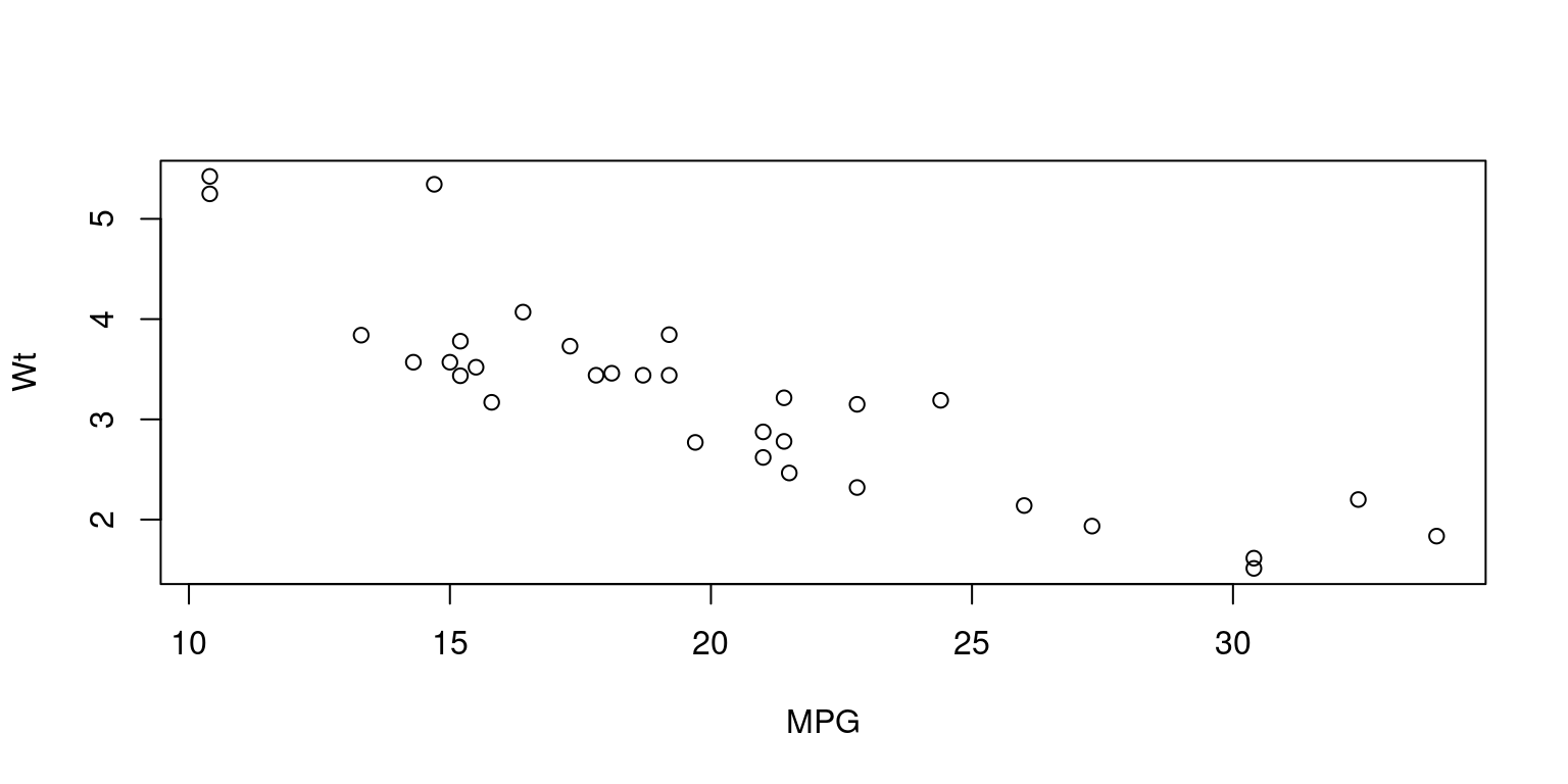
Assessing the Relationship using Scatter Plot

# Load the mtcars dataset
data(mtcars)
# relationship between the mpg and wt variables
plot(mtcars$mpg, mtcars$wt, xlab = "MPG", ylab = "Wt")

Correlation Matrix

  1. The correlation coefficients between two variables are displayed in a table called a correlation matrix.

  2. It is a symmetric matrix where the upper and lower triangles hold the correlation coefficients between each pair of variables, and the diagonal holds the correlation of each variable with itself, which is always 1.

  3. It is an effective tool for investigating the connections between variables in a dataset.

Creating a Correlation Matrix in R

# Load the mtcars dataset
data(mtcars)
# Calculate the correlation matrix for mpg, wt, hp, drat
cor(mtcars[,c("mpg","wt","hp","drat")])
            mpg         wt         hp       drat
mpg   1.0000000 -0.8676594 -0.7761684  0.6811719
wt   -0.8676594  1.0000000  0.6587479 -0.7124406
hp   -0.7761684  0.6587479  1.0000000 -0.4487591
drat  0.6811719 -0.7124406 -0.4487591  1.0000000

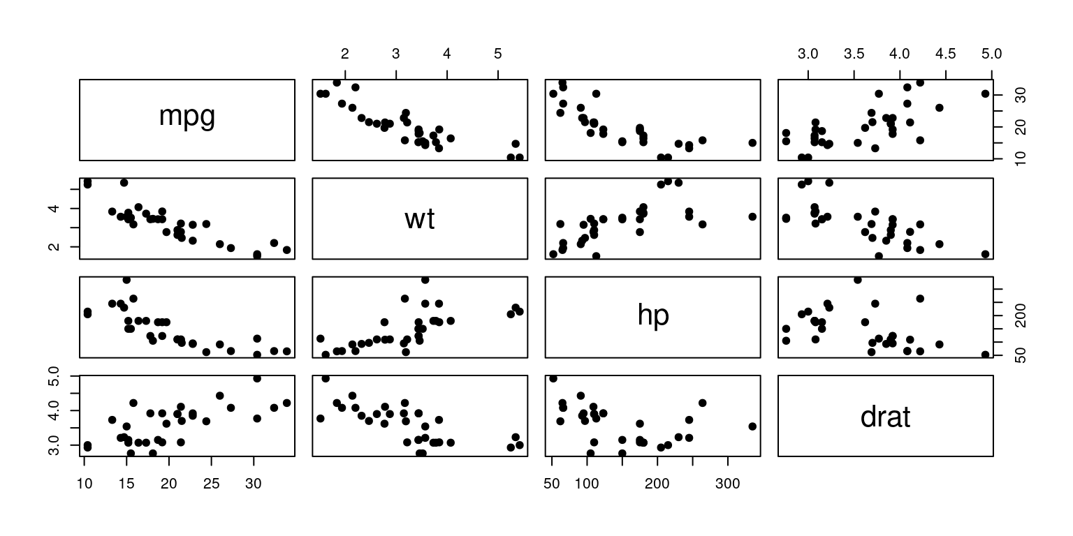
Creating a Scatter Plot Matrix in R

# Load the mtcars dataset
data(mtcars)
# scatter plot matrix for mpg, wt, hp, drat
pairs(mtcars[,c("mpg","wt","hp","drat")], pch = 19)

Hypothesis Testing for Correlation

The hypothesis testing process can be used to examine the null hypothesis that there is no significant correlation between two variables using Pearson’s correlation coefficient:

  1. State the null hypothesis (H0) and the alternative hypothesis (H1):
  • H0: There is no significant correlation between the two variables (the correlation coefficient is zero).

  • H1: There is a significant correlation between the two variables (the correlation coefficient is not zero).

  1. Determine the level of significance (\(α\)) that you will use to test the hypothesis.
  2. Calculate the sample correlation coefficient (\(r\)) and the sample size (\(n\)).
  3. Calculate the degrees of freedom (\(df\)), which is equal to \(n-2\).
  4. Calculate the critical values for the test statistic, using a table or calculator based on the significance level and degrees of freedom.
  5. Calculate the test statistic (\(t\)), which is equal to \(r\sqrt{df/(1-r^2)}\).
  6. Compare the test statistic to the crucial values. Reject the null hypothesis if the test statistic is outside the crucial range. Reject the null hypothesis if the test statistic is inside the crucial range.
  7. Calculate a p-value for the test statistic.
    • Reject the null hypothesis if the p-value is less than the significance level.

    • Fail to reject the null hypothesis if the p-value exceeds the significance level.

Hypothesis Test for Pearson’s correlation coefficient in R

  1. Run the following code using cor.test()
# Load the mtcars dataset
data(mtcars)
# Perform a hypothesis test for the correlation between mpg and wt
cor.test(mtcars$mpg, mtcars$wt)

    Pearson's product-moment correlation

data:  mtcars$mpg and mtcars$wt
t = -9.559, df = 30, p-value = 1.294e-10
alternative hypothesis: true correlation is not equal to 0
95 percent confidence interval:
 -0.9338264 -0.7440872
sample estimates:
       cor 
-0.8676594 
  • This will execute a hypothesis test and calculate the Pearson correlation coefficient, returning the test statistic, degrees of freedom, p-value, and correlation coefficient confidence interval.

  • We can reject the null hypothesis and determine that there is a significant correlation between the two variables if the p-value is smaller than the significance level.

  1. Alternately, the corr.test() function, part of the psych package, can be used to perform hypothesis testing and confidence interval estimation for Pearson’s correlation coefficient.
# Load the mtcars dataset
data(mtcars)

# Calculate the correlation between mpg and wt
library(psych)
corr.test(mtcars$mpg, 
          mtcars$wt, 
          method = "pearson", 
          use = "pairwise", 
          adjust = "none", 
          ci = TRUE, 
          alpha = 0.05)
Call:corr.test(x = mtcars$mpg, y = mtcars$wt, use = "pairwise", method = "pearson", 
    adjust = "none", alpha = 0.05, ci = TRUE)
Correlation matrix 
[1] -0.87
Sample Size 
[1] 32
[1] 0

 To see confidence intervals of the correlations, print with the short=FALSE option
  • This will return the correlation coefficient, p-value, and confidence interval for the correlation between mpg and wt.

  • The output will also include information on the sample size, missing values, and adjustment method used.

  • To use the corr.test() function on a dataframe in R, it is helpful to first select the columns of interest and pass them as arguments to the function.

# Load the mtcars dataset
data(mtcars)

# Select the columns of interest
vars <- c("mpg", "disp", "hp", "wt")

# Calculate the correlation matrix and perform hypothesis tests
library(psych)
corr.test(mtcars[, vars], 
          method = "pearson", 
          use = "pairwise", 
          adjust = "none", 
          ci = TRUE, 
          alpha = 0.05)
Call:corr.test(x = mtcars[, vars], use = "pairwise", method = "pearson", 
    adjust = "none", alpha = 0.05, ci = TRUE)
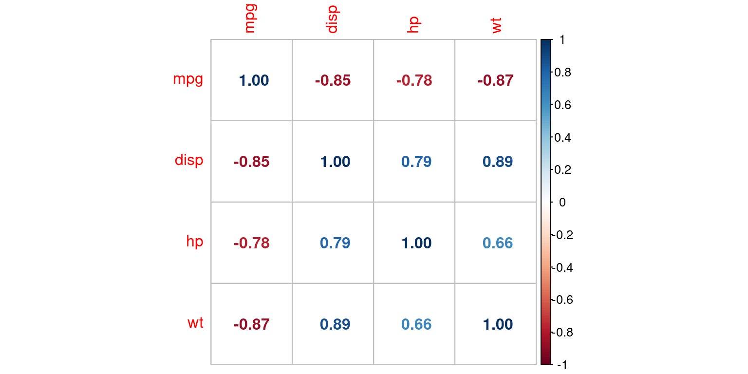
Correlation matrix 
       mpg  disp    hp    wt
mpg   1.00 -0.85 -0.78 -0.87
disp -0.85  1.00  0.79  0.89
hp   -0.78  0.79  1.00  0.66
wt   -0.87  0.89  0.66  1.00
Sample Size 
[1] 32
Probability values (Entries above the diagonal are adjusted for multiple tests.) 
     mpg disp hp wt
mpg    0    0  0  0
disp   0    0  0  0
hp     0    0  0  0
wt     0    0  0  0

 To see confidence intervals of the correlations, print with the short=FALSE option
  • In this example, the names of the relevant columns from the mtcars dataset are contained in a character vector in the vars variable. The mtcars dataset subset containing only these columns is subsequently submitted to the corr.test() function.

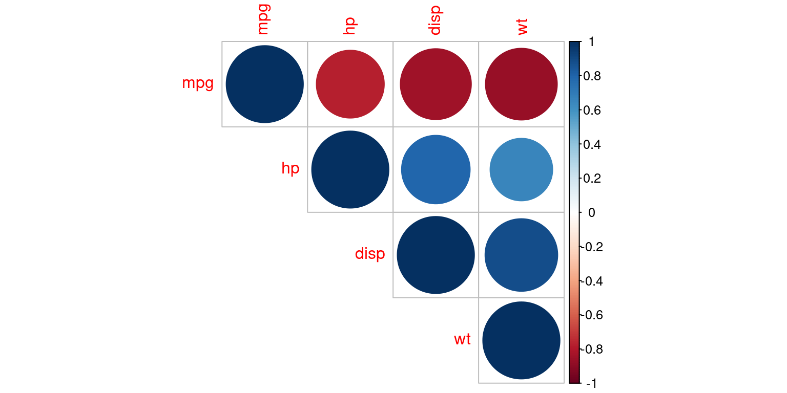
  • The result will be a correlation matrix with rows and columns matching to the relevant variables, as well as a set of hypothesis tests.

  • The hypothesis tests will report the correlation coefficient, p-value, and confidence range for each correlation, and the matrix will display the pairwise correlations between the variables.

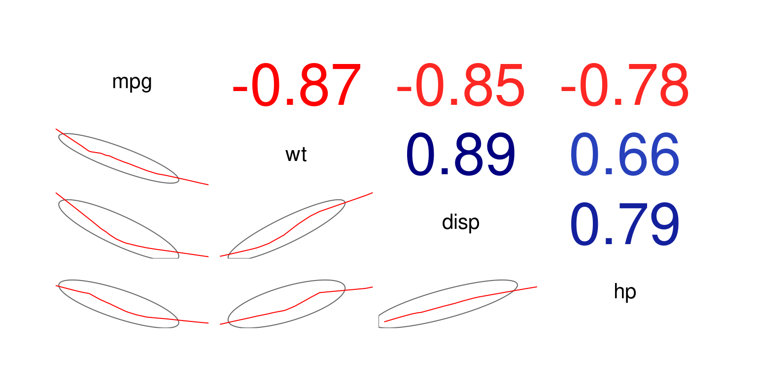
Visualizing Correlation Matrix using corrgram

# Load the mtcars dataset
data(mtcars)
# Select the columns of interest
vars <- c("mpg", "disp", "hp", "wt")

# Calculate the correlation matrix and perform hypothesis tests
library(corrgram)

# Create the corrgram plot
corrgram(mtcars[, vars],
         order = TRUE, 
         lower.panel = panel.ellipse, 
         upper.panel = panel.cor)
Warning in par(usr): argument 1 does not name a graphical parameter

Warning in par(usr): argument 1 does not name a graphical parameter

Warning in par(usr): argument 1 does not name a graphical parameter

Warning in par(usr): argument 1 does not name a graphical parameter

Warning in par(usr): argument 1 does not name a graphical parameter

Warning in par(usr): argument 1 does not name a graphical parameter

Visualizing Correlation Matrix using corrplot

# Load the mtcars dataset
data(mtcars)
library(corrplot)
corrplot 0.92 loaded
# Select the columns of interest
vars <- c("mpg", "disp", "hp", "wt")
M <- cor(mtcars[, vars])
corrplot(M, type="upper", order="hclust")

Visualizing Correlation Matrix using corrplot

# Load the mtcars dataset
data(mtcars)
library(corrplot)
# Select the columns of interest
vars <- c("mpg", "disp", "hp", "wt")
M <- cor(mtcars[, vars]) 
corrplot(M, method="number")

Spearman’s Correlation

Assumptions in Pearson’s Correlation Coefficient

Pearson’s correlation coefficient is a parametric measure of the linear relationship between two variables. It relies on several assumptions, including:

  1. Linearity: The two variables’ relationship should be linear. The Pearson’s correlation coefficient may not adequately represent the strength of the association between the variables if the relationship is nonlinear.

  2. Normality: The correlated variables should have a normal distribution. The reliability of Pearson’s correlation coefficient may be compromised if the variables are not normally distributed.

  3. Homoscedasticity: All levels of the variables should have the same variance for the two variables. The Pearson correlation coefficient may be impacted by unequal variance, making the relationship between the variables look stronger or weaker than it actually is.

  4. Independence: The two variables need to be unrelated to one another. The Pearson correlation coefficient may not effectively depict the relationship between the variables if the two variables are not independent.

  5. Outliers: The correlation coefficient might be distorted by outliers, which can affect the outcomes. As a result, it is advised to check the data for outliers prior to determining the Pearson’s correlation coefficient.

Before using Pearson’s correlation coefficient, it is essential to validate these hypotheses to avoid incorrect interpretations of the data. Where these assumptions are not true, nonparametric correlation measurements, such as Spearman’s correlation coefficient, may be more appropriate.

Spearman’s Correlation Coefficient

  1. A nonparametric indicator of the relationship between two variables is the Spearman correlation. It evaluates how well a monotonic function, which can only be strictly increasing or decreasing, can describe the relationship between two variables.

  2. It is independent of the distributional assumptions underlying the correlated variables.

  3. Instead, it computes the correlation coefficient based on the ranks of the variables, rather than their actual values.

Calculating Spearman’s Correlation Coefficient in R

# Load a dataset
data(mtcars)
# Calculate the Spearman correlation between mpg and wt
cor(mtcars$mpg, 
    mtcars$wt, 
    method = "spearman")
[1] -0.886422

References

[1]

Hair, J. F., Jr., Bush, R. P., & Ortinau, D. J. (2020). Essentials of marketing research. McGraw-Hill Education.

[2]

Smith, J. K., Johnson, L. M., & Brown, E. F. (2020). Correlates of sleep quality in college students. Journal of Sleep Research, 29(3), e12950. https://doi.org/10.1111/jsr.12950

[3]

Cohen, J., Cohen, P., West, S. G., & Aiken, L. S. (2003). Applied multiple regression/correlation analysis for the behavioural sciences (3rd ed.). Erlbaum.

[4]

Garcia, M. A. (2018). Correlates of academic performance in high school students: A study of demographic and psychological factors (Doctoral dissertation). University of California, Los Angeles.

[5]

Gupta, R., Shah, P., & Desai, P. (2020). Correlation between body mass index and sleep duration in young adults. Journal of Clinical Sleep Medicine, 16(2), 287–292. https://doi.org/10.5664/jcsm.8120

[6]

Chang, C.-C., & Lin, C.-J. (2011). LIBSVM: A library for support vector machines. In ACM Transactions on Intelligent Systems and Technology (Vol. 2, No. 3, Article 27). https://doi.org/10.1145/1961189.1961199

[7]

Centers for Disease Control and Prevention. (2022). Coronary heart disease (CHD). https://www.cdc.gov/heartdisease/coronary_ad.htm

[8]

Chung, J. Y., & Yi, Y. (2019). The impact of user-generated content on consumer purchase behavior: An empirical investigation of supply-side antecedents. Journal of Interactive Marketing, 46, 74-87. https://doi.org/10.1016/j.intmar.2018.12.001

[9]

Kumar, V., & Pansari, A. (2016). Measuring brand value co-creation: Conceptualization, scale development, and validation. In Proceedings of the 2016 Winter Marketing Educators’ Conference (pp. 45-46). American Marketing Association.

[10]

Wang, D., & Yang, J. (2021). Correlation risk and asset pricing: Evidence from the Chinese stock market. Finance Research Letters, 38, 101749. https://doi.org/10.1016/j.frl.2020.101749

[11]

Chen, L., & Jiang, Y. (2017). Correlation between stock returns and investor sentiment: Evidence from the Chinese stock market. In Proceedings of the 2017 International Conference on Management Science and Management Innovation (pp. 118-124). Atlantis Press.

[12]

Hull, J. C. (2017). Options, futures, and other derivatives (10th ed.). Pearson.

[13]

Fedorov, V. V., & Zelen, M. (2019). Correlation in regression with censored survival data. Statistical Methods in Medical Research, 28(8), 2402-2415. https://doi.org/10.1177/0962280218787804

[14]

García-Pérez, A., & Sánchez-Matilla, R. (2018). On the relationship between standard deviation and mean in the correlation coefficient. In Proceedings of the 9th International Conference on Applied Human Factors and Ergonomics (pp. 102-108). Springer.

[15]

Derrick, B., & Whitehead, A. (2019). Understanding correlation: Factors that affect the size and direction of r. Routledge.

[16]

Taha, H. A., & Saad, M. A. (2021). Pearson correlation coefficients: How to interpret and report them in medical research studies. Journal of Medical Research and Practice, 10(2), 49-55. https://doi.org/10.3126/jmrp.v10i2.35757

[17]

Brendel, K. E. (2019). Pearson correlation analysis of student retention in online learning. In Proceedings of the 2019 International Conference on Distance Education and E-Learning (pp. 70-75). ACM.

[18]

Aron, A., Coups, E. J., & Aron, E. N. (2019). Statistics for psychology (7th ed.). Pearson.

[19]

Al-Adwan, A. S. (2020). Spearman’s rank correlation coefficient: A guide for medical researchers. Journal of Health and Medical Sciences, 3(2), 147-155. https://doi.org/10.35500/jhms.2020.3.2.14

[20]

Diaz-Uriarte, R. (2019). Spearman’s rank correlation coefficient: A review and some new results. In Proceedings of the 2019 International Conference on Computational Statistics and Data Science (pp. 106-111). Springer.

[21]

Bluman, A. G. (2017). Elementary statistics: A step by step approach (10th ed.). McGraw-Hill.

[22]

Smith, J. A., & Jones, B. D. (2018). Hypothesis testing in correlation analysis: A review of current practices and recommendations for improvement. Journal of Applied Statistics, 45(9), 1645-1656. https://doi.org/10.1080/02664763.2017.1413485

[23]

Gupta, R. K., & Sharma, M. (2020). A hypothesis testing framework for nonparametric correlation measures. In Proceedings of the 2020 International Conference on Data Science, E-learning and Information Systems (pp. 12-17). IEEE.

[24]

Book: Field, A., Miles, J., & Field, Z. (2012). Discovering statistics using R. Sage.

[25]

Mishra, D., & Routray, S. (2021). Analyzing spatial patterns and temporal trends of air pollution using correlogram and time series analysis. Journal of Environmental Management, 295, 113107. https://doi.org/10.1016/j.jenvman.2021.113107

[26]

Lebeau, T., & Elouedi, Z. (2019). A comparative study of the correlogram and the principal component analysis in a remote sensing application. In Proceedings of the 2019 International Conference on Image and Vision Computing New Zealand (pp. 1-6). IEEE.

[27]

Chatfield, C. (2004). The analysis of time series: An introduction (6th ed.). CRC Press.

[28]

Wang, Y., & Song, J. (2021). Analysis of the relationship between macroeconomic variables and real estate prices in China using corrplot. Applied Economics Letters, 28(5), 408-413. https://doi.org/10.1080/13504851.2020.1806448

[29]

Sarathchandran, P. S., & Prasanth, K. (2019). Correlation analysis of biometric traits using corrplot. In Proceedings of the 2019 International Conference on Machine Learning, Big Data, Cloud and Parallel Computing (pp. 58-62). ACM.

[30]

Lehtonen, R., & Pahkinen, E. (2004). Practical methods for design and analysis of complex surveys (2nd ed.). Wiley.

[31]

Wu, H., Chen, C., & Su, H. (2020). Development of a correlation matrix-based evaluation model for water quality in river systems. Environmental Science and Pollution Research, 27(22), 28090-28102. https://doi.org/10.1007/s11356-020-09483-6

[32]

Oriabure, E., & Jimoh, R. G. (2020). Correlation matrix analysis of socio-economic variables and energy consumption in Nigeria. In Proceedings of the 2020 International Conference on Sustainable Energy and Green Technology (pp. 1-7). IEEE.

[33]

Gelman, A., & Hill, J. (2006). Data analysis using regression and multilevel/hierarchical models. Cambridge University Press.